This project looks at how long patients survived in the Veterans Administration lung cancer trial, a classic dataset for time-to-event modelling in R. The goal is to compare standard and experimental chemotherapy while walking through a full Cox proportional hazards workflow: exploratory survival curves, adjusted modelling, and model checks.
Survival analysis is useful when what matters is not just whether an event happened, but when. Here the event is death, and the methods account for censoring and for differences in how long each patient was followed.
The dataset covers 137 male patients with advanced, inoperable lung cancer, randomised to standard or experimental treatment. It is small enough to work through end to end, but rich enough to show the main decisions a real survival analysis involves.
The project comes in two parts:
Overview: this page, a high-level summary of the key findings and visuals.
Full Report: the step-by-step analysis, model building, and diagnostics.
Study Overview
# KM medians overall and by armkm_all <-survfit(Surv(time, status) ~1, data = veteran2)km_by <-survfit(Surv(time, status) ~ trt, data = veteran2)overall <-surv_median(km_all)byarm <-surv_median(km_by)med_all <-round(overall$median)ci_all_l <-round(overall$lower); ci_all_u <-round(overall$upper)med_std <-round(byarm$median[byarm$strata =="trt=Standard"])ci_std_l <-round(byarm$lower [byarm$strata =="trt=Standard"])ci_std_u <-round(byarm$upper [byarm$strata =="trt=Standard"])med_exp <-round(byarm$median[byarm$strata =="trt=Experimental"])ci_exp_l <-round(byarm$lower [byarm$strata =="trt=Experimental"])ci_exp_u <-round(byarm$upper [byarm$strata =="trt=Experimental"])# Baseline summariesn_total <-nrow(veteran2)n_by_trt <- veteran2 %>%count(trt, name ="n")n_std_n <- n_by_trt$n[n_by_trt$trt =="Standard"]n_exp_n <- n_by_trt$n[n_by_trt$trt =="Experimental"]q_age <-quantile(veteran2$age, probs =c(0.25, 0.5, 0.75))q_karno <-quantile(veteran2$karno, probs =c(0.25, 0.5, 0.75))med_age <-round(q_age[2]); iqr_age_l <-round(q_age[1]); iqr_age_u <-round(q_age[3])med_karno <-round(q_karno[2]); iqr_kar_l <-round(q_karno[1]); iqr_kar_u <-round(q_karno[3])cell_pct <-round(100*prop.table(table(veteran2$celltype)), 1)prior_pct <-round(100*prop.table(table(veteran2$prior)), 1)prior_yes <-unname(prior_pct["Yes"])lr <-survdiff(Surv(time, status) ~ trt, data = veteran2)lr_p <-signif(1-pchisq(lr$chisq, length(lr$n) -1), 3)deaths <-sum(veteran2$status ==1)censored <-sum(veteran2$status ==0)deaths_pct <-round(100* deaths / n_total, 1)cens_pct <-round(100* censored / n_total, 1)cat(glue("**Study population**- {n_total} male patients; Standard = **{n_std_n}**, Experimental = **{n_exp_n}**- Median age: **{med_age}** years (IQR: {iqr_age_l} to {iqr_age_u})- Median Karnofsky score: **{med_karno}** (IQR: {iqr_kar_l} to {iqr_kar_u})- Cell type: Squamous {cell_pct['Squamous']}%, Small cell {cell_pct['Small cell']}%, Adenocarcinoma {cell_pct['Adenocarcinoma']}%, Large cell {cell_pct['Large cell']}%- Prior therapy: **{prior_yes}%** yes**Survival outcomes**- Median survival (all): **{med_all}** days (95% CI: {ci_all_l} to {ci_all_u})- Standard arm: **{med_std}** days (95% CI: {ci_std_l} to {ci_std_u})- Experimental arm: **{med_exp}** days (95% CI: {ci_exp_l} to {ci_exp_u})- Log-rank *p* = **{lr_p}****Events**- Deaths: **{deaths}** ({deaths_pct}%) | Censored: **{censored}** ({cens_pct}%)"))
**Study population**
- 137 male patients; Standard = **69**, Experimental = **68**
- Median age: **62** years (IQR: 51 to 66)
- Median Karnofsky score: **60** (IQR: 40 to 75)
- Cell type: Squamous 25.5%, Small cell 35%,
  Adenocarcinoma 19.7%, Large cell 19.7%
- Prior therapy: **29.2%** yes

**Survival outcomes**
- Median survival (all): **80** days (95% CI: 52 to 105)
- Standard arm: **103** days (95% CI: 59 to 132)
- Experimental arm: **52** days (95% CI: 44 to 95)
- Log-rank *p* = **0.928**

**Events**
- Deaths: **128** (93.4%) | Censored: **9** (6.6%)
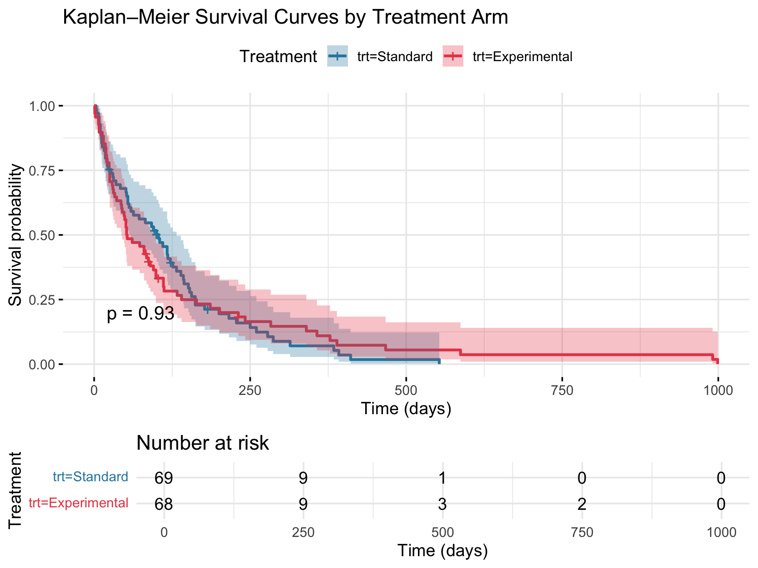
Survival by Treatment Group
The trial’s main question: does the experimental regimen improve survival over standard chemotherapy?
The survival curves for the two treatment arms overlap almost entirely throughout follow-up. The log-rank test confirms no statistically significant difference (p = 0.928). The experimental chemotherapy did not improve survival in this cohort.
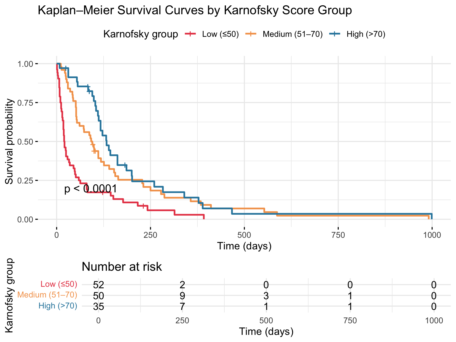
Survival by Karnofsky Performance Score
Karnofsky score is a 0 to 100 measure of functional status. In this dataset it is one of the clearest predictors of survival.
The separation between the groups is clear: patients with higher functional status survived much longer than those with lower scores. That pattern is strong, consistent, and carries through to the adjusted Cox model, where Karnofsky score is the most important predictor in the analysis.
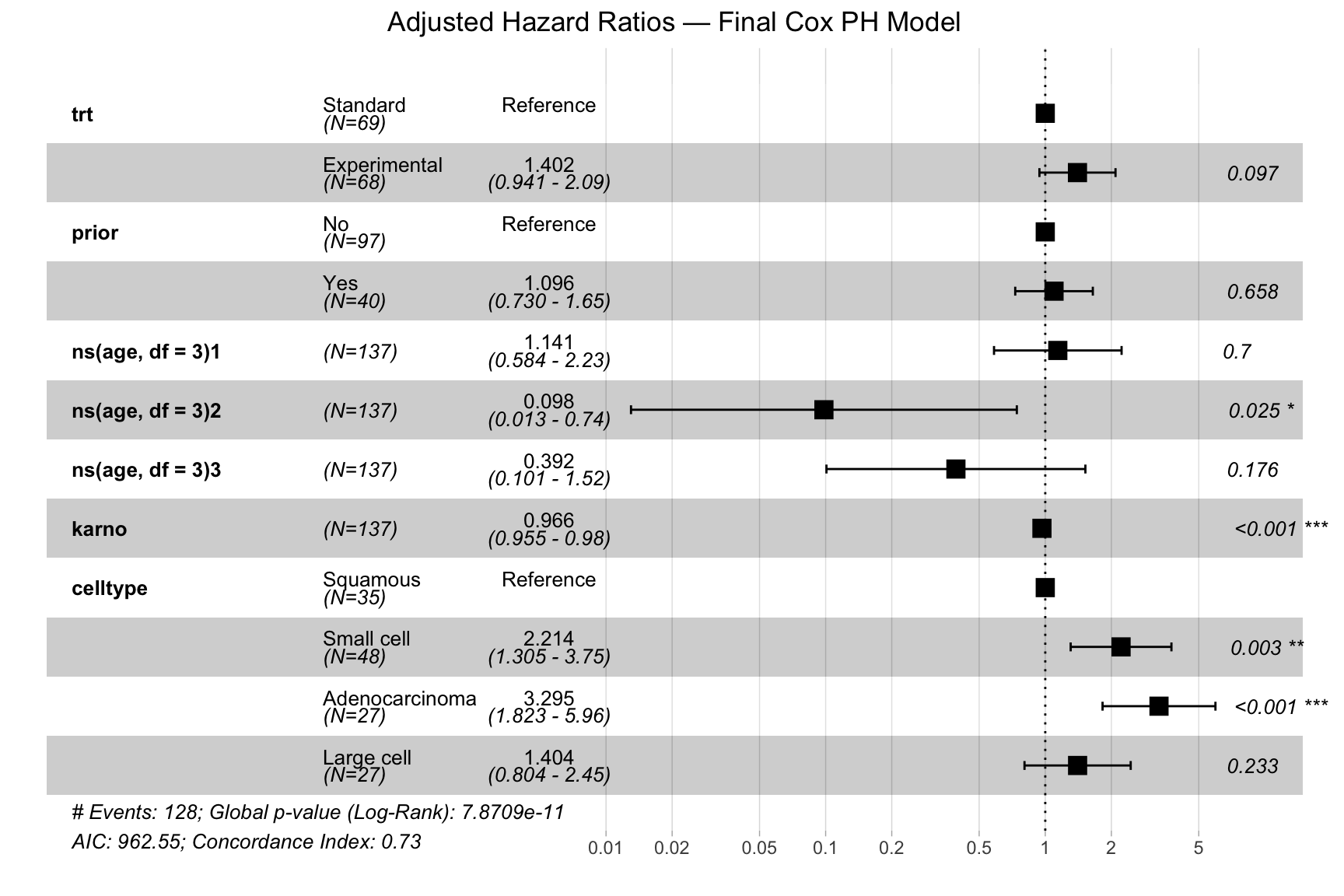
Final Cox Model: Adjusted Hazard Ratios
This plot shows the final adjusted Cox model: treatment group, prior therapy, age, Karnofsky score, and cell type.
The clearest signals in the model are Karnofsky score and tumour cell type. Higher Karnofsky scores are associated with lower risk, while adenocarcinoma and small cell carcinoma show substantially higher hazard than squamous cell carcinoma. Even after adjustment, the treatment effect remains modest and uncertain (HR ≈ 1.4, p = 0.097). Overall, the model discriminates much better than a treatment-only model, with concordance improving from about 0.51 to 0.74.
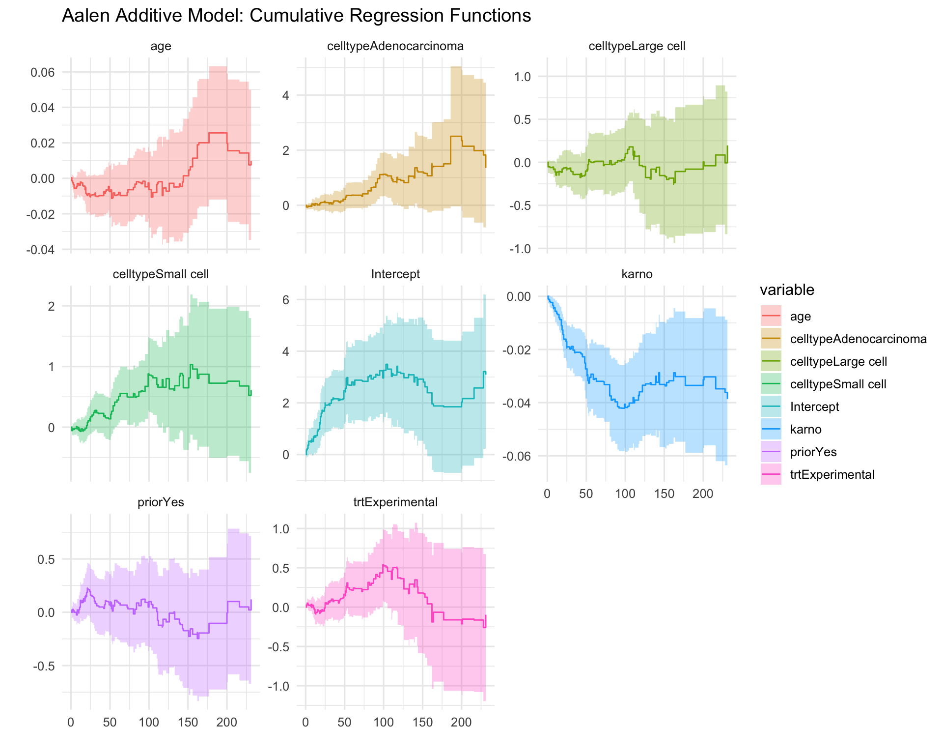
Aalen Additive Model: Time-Varying Effects
This plot rechecks the main findings using an additive survival model instead of the Cox model.
The result is broadly the same. Karnofsky score remains the strongest and most stable predictor of survival, while treatment group and prior therapy contribute little on their own. Seeing the same pattern across two different modelling approaches adds confidence to the overall interpretation.