Fatal Motorcycle Crashes

A sub-analysis of the ARDD focusing on fatal motorcycle crashes.

Motorcycling offers freedom and convenience, but the safety risk is still high relative to other road users. Even with better bikes and better gear, motorcyclists remain overrepresented in fatal crash data in Australia.

This sub-analysis investigates trends in fatal crashes involving motorcyclists and pillion passengers, drawing on over three decades of data. It aims to identify persistent risk patterns by year, state, and rider population, and to assess the relative burden on motorcyclists compared to their licensed population base.

1. Key Findings

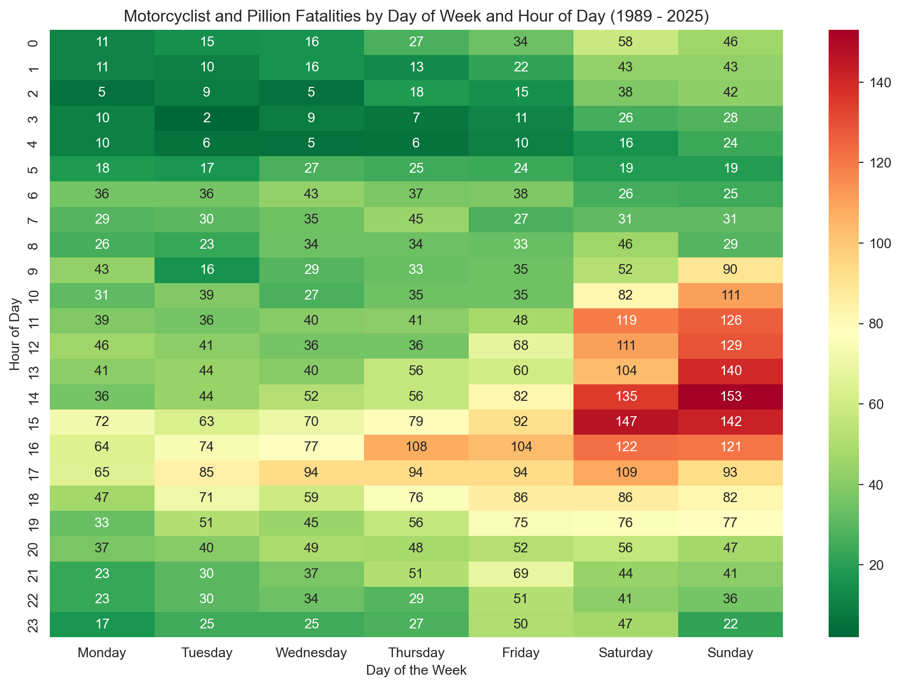
Time and Day Matter (A Lot) Fatalities peak sharply on Saturdays and Sundays, particularly in the afternoon hours between 1 PM and 5 PM. This aligns with recreational riding patterns, where less experienced or infrequent riders may be pushing limits on unfamiliar or technical roads (“the twisties”).
Single-Vehicle vs Multi-Vehicle Crashes A sizeable proportion of fatal crashes involve single vehicles, particularly on weekends. This supports the idea that weekend fatalities may disproportionately involve loss of control rather than collision with another vehicle—an angle worth further exploration.
Gender Disparity 93.7% of fatalities were male, reflecting both exposure and likely differences in riding patterns and risk behaviour.
Age Distribution Fatalities skew young, peaking in the early 20s, then tapering with age—though a surprising number of older riders (60+) are still represented. The age distribution for female fatalities shows a bimodal pattern, possibly reflecting pillion vs rider roles.
Seasonal Variation Fatalities are higher in summer and spring, peaking in March, and lowest in the winter months, especially July. Not exactly surprising—cold rain is a great motivator to leave the bike parked—but the difference is notable.

2. Data Cleaning

The notebook uses full_clean_pipeline() from scripts/data_cleaning.py to load and tidy the raw crash data — handling missing values, dropping redundant columns, and returning a clean, analysis-ready DataFrame. The dataset is then filtered to isolate fatal incidents involving motorcycle riders and pillion passengers.

Code

"""
This notebook is fully self-contained and does not depend on the main EDA notebook.
The dataset is loaded and cleaned using `full_clean_pipeline()` from `scripts/data_cleaning.py`, which:
- Loads raw data from /data/Crash_Data.csv
- Cleans missing values and harmonizes variables
- Drops incomplete or irrelevant columns
- Returns a tidy, ready-to-analyze DataFrame
"""

# Set the directory for the script
import sys
sys.path.append("../scripts")

# Importing necessary libraries
import pandas as pd
import numpy as np
import matplotlib.pyplot as plt
import seaborn as sns
from IPython.display import display
from data_cleaning import full_clean_pipeline

df = pd.read_csv("../data/Crash_Data.csv", low_memory=False)
df = full_clean_pipeline(df)

# Create variable for the earliest and latest years in the dataset to be dynamically displayed in plot titles
latest_year = df['Year'].max()
earliest_year = df['Year'].min()
print(f"The dataset contains data from {earliest_year} to {latest_year}.")

# Define constants for reuse
month_names = {
    1: 'January', 2: 'February', 3: 'March', 4: 'April', 5: 'May', 6: 'June',
    7: 'July', 8: 'August', 9: 'September', 10: 'October', 11: 'November', 12: 'December'
}
month_order = [
    'January', 'February', 'March', 'April', 'May', 'June',
    'July', 'August', 'September', 'October', 'November', 'December'
]
day_order = ['Monday', 'Tuesday', 'Wednesday', 'Thursday', 'Friday', 'Saturday', 'Sunday']
custom_palette = {'Female': 'lightcoral', 'Male': 'skyblue'}

# Filter for Motorcyclists and Pillion Passengers
motorcyclist_pillion_fatalities = df[df['Road User'].isin(['Motorcycle rider', 'Motorcycle pillion passenger'])]
motorcyclist_fatalities = df[df['Road User'] == 'Motorcycle rider']
pillion_fatalities = df[df['Road User'] == 'Motorcycle pillion passenger']

# print("\nFiltered DataFrames created:")
# print(f"- motorcyclist_pillion_fatalities: {motorcyclist_pillion_fatalities.shape[0]} rows")
# print(f"- motorcyclist_fatalities: {motorcyclist_fatalities.shape[0]} rows")
# print(f"- pillion_fatalities: {pillion_fatalities.shape[0]} rows")
# print("\nMissing values in motorcyclist_pillion_fatalities:")
# print(motorcyclist_pillion_fatalities.isnull().sum())
# print("\nMissing values in motorcyclist_fatalities:")
# print(motorcyclist_fatalities.isnull().sum())
# print("\nMissing values in pillion_fatalities:")
# print(pillion_fatalities.isnull().sum())

The dataset contains data from 1989 to 2025.

3. Data Visualisation

The sections below explore how motorcycle fatalities vary by time, geography, and rider demographics, and situate the death toll against the licensed rider population.

3.1 Yearly Fatalities

Code

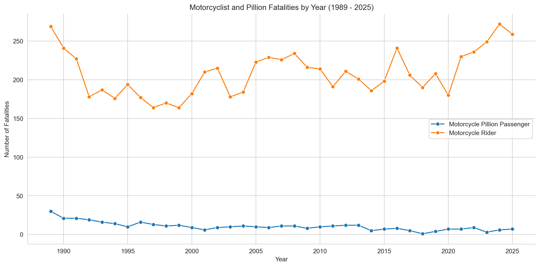
# Group data by Year and Road User for the filtered set
fatalities_by_year_user = motorcyclist_pillion_fatalities.groupby(['Year', 'Road User'])['Crash ID'].count().reset_index(name='Fatalities')

# Capitalize the legend labels
fatalities_by_year_user['Road User'] = fatalities_by_year_user['Road User'].str.title()

# Plotting raw numbers of Fatalities
sns.set_style('whitegrid')
plt.figure(figsize=(12, 6))
sns.lineplot(x='Year', 
            y='Fatalities',
            data=fatalities_by_year_user, 
            hue='Road User', 
            marker="o")
plt.title(f'Motorcyclist and Pillion Fatalities by Year ({earliest_year} - {latest_year})')
plt.xlabel('Year')
plt.ylabel('Number of Fatalities')
plt.grid(True)
sns.despine()
plt.legend(title=None)  # ← Removes legend title
plt.tight_layout()
plt.show()

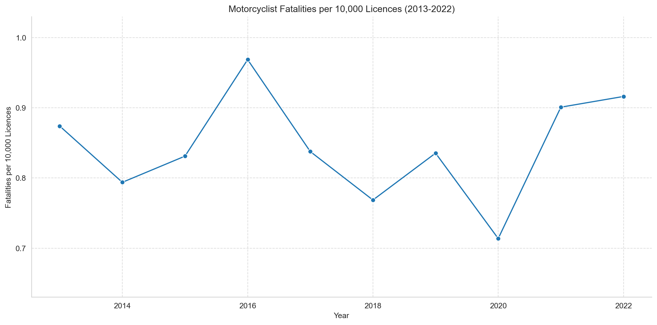
Raw fatality counts have remained broadly flat — pillion deaths are relatively stable, and rider deaths show no meaningful long-term decline. But with Australia’s population and licensed rider base both growing since 1989, raw numbers can be misleading. Normalising fatalities per 10,000 motorcycle licences offers a more meaningful picture of risk over time. Licensing data from BITRE is available from 2013, so the chart below covers that window.

Integrating Motorcycle Licence Data

BITRE publishes annual motorcycle licensing data in its Australian Infrastructure and Transport Statistics Yearbook (Road chapter), split across Full, Provisional, and L Permit tiers. The relevant file is bitre-yearbook-YYYY-04-road.xlsx. The data needs some cleanup (removing non-data rows, forward-filling tier labels, and reshaping) before it can be merged with crash counts, but the result gives a more useful risk metric than raw fatalities alone.

Code

def analyze_motorcycle_fatality_rates(fatalities_df):
    """
    Load motorcycle license data and calculate fatality rates per 10,000 licences.
    Returns the prepared dataframe for plotting.
    """
    # 1. Load and process licence data
    # Source: BITRE Australian Infrastructure and Transport Statistics Yearbook, Road chapter.
    # Annual Excel file: bitre-yearbook-YYYY-04-road.xlsx ("Drivers licences" table).
    # Latest edition: https://www.bitre.gov.au/sites/default/files/documents/bitre-yearbook-2025-04-road.xlsx
    df_licenses = pd.read_csv("../data/motorcycle_licenses.csv", header=None, skiprows=1, skipinitialspace=True)

    # Define known licence tier labels
    tiers = ["Full licence", "Provisional licence", "L Permits"]

    # Add a column to track the tier label
    df_licenses["tier"] = df_licenses[0].where(df_licenses[0].isin(tiers)).ffill()

    # Filter out rows that are just the tier labels themselves
    df_licenses = df_licenses[~df_licenses[0].isin(tiers)].copy()

    # Rename columns based on expected positions
    if df_licenses.shape[1] == 9:  # 8 original + 1 tier
        df_licenses.columns = [
            "date", "car", "motorcycle", "light_rigid",
            "medium_rigid", "heavy_rigid", "heavy_combination",
            "multi_combination", "tier"
        ]
    else:
        print(
            f"Warning: Unexpected number of columns ({df_licenses.shape[1]}) "
            "in license data after adding tier. Check CSV structure."
        )
        return pd.DataFrame(), 2013, 2022

    # Extract the last two digits after the hyphen
    two_digit_year = df_licenses["date"].str.extract(r"-(\d{2})$").iloc[:, 0]

    # Prepend '20' and convert to numeric (integer), handling potential errors
    df_licenses["year"] = pd.to_numeric("20" + two_digit_year, errors='coerce')

    # Clean the motorcycle licence count column
    df_licenses["motorcycle"] = (
        df_licenses["motorcycle"]
        .astype(str)
        .str.replace(",", "", regex=False)
        .str.replace(" ", "", regex=False)
        .str.strip()
        .replace("", pd.NA)
    )

    # Convert motorcycle column to numeric, coercing errors to NA
    df_licenses["motorcycle"] = pd.to_numeric(df_licenses["motorcycle"], errors="coerce")

    # Drop rows where year extraction failed or motorcycle count is missing/invalid
    df_licenses = df_licenses.dropna(subset=["year", "motorcycle"])

    # Convert year and motorcycle count to integer type now that NAs are handled
    if df_licenses.empty:
        print("Warning: Licence DataFrame is empty after cleaning and dropping NAs. Cannot create summary.")
        return pd.DataFrame(), 2013, 2022

    df_licenses["year"] = df_licenses["year"].astype(int)
    df_licenses["motorcycle"] = df_licenses["motorcycle"].astype(int)

    # Group by year and sum the motorcycle licences across all tiers
    license_summary = (
        df_licenses.groupby("year")["motorcycle"]
        .sum()
        .reset_index(name="total_motorcycle_licenses")
    )

    # 2. Calculate total fatalities per year (riders only, excluding pillion passengers)
    total_fatalities_per_year = (
        fatalities_df.groupby('Year')['Crash ID']
        .count()
        .reset_index(name='total_fatalities')
    )

    # 3. Merge fatality data with licence data
    merged_data = pd.merge(
        total_fatalities_per_year,
        license_summary,
        left_on='Year',
        right_on='year',
        how='inner'
    )

    # 4. Filter for the desired year range
    start_year_rate = 2013
    end_year_rate = 2022
    merged_data_filtered = merged_data[
        (merged_data['Year'] >= start_year_rate) & (merged_data['Year'] <= end_year_rate)
    ].copy()

    # 5. Calculate the rate per 10,000 licences
    merged_data_filtered['fatalities_per_10k_licenses'] = np.where(
        merged_data_filtered['total_motorcycle_licenses'] > 0,
        (merged_data_filtered['total_fatalities'] / merged_data_filtered['total_motorcycle_licenses']) * 10000,
        0
    )

    return merged_data_filtered, start_year_rate, end_year_rate


# Run the analysis function (riders only — pillion passengers excluded as they don't hold motorcycle licences)
merged_data_filtered, start_year_rate, end_year_rate = analyze_motorcycle_fatality_rates(motorcyclist_fatalities)

# Plot the rate over time
if not merged_data_filtered.empty:
    plt.figure(figsize=(12, 6))
    sns.lineplot(
        x='Year',
        y='fatalities_per_10k_licenses',
        data=merged_data_filtered,
        marker='o'
    )
    plt.title(f'Motorcyclist Fatalities per 10,000 Licences ({start_year_rate}-{end_year_rate})')
    plt.xlabel('Year')
    plt.ylabel('Fatalities per 10,000 Licences')
    plt.yticks(np.arange(0.7, 1.01, 0.1))
    plt.ylim(0.63, 1.03)
    plt.grid(True, linestyle='--', alpha=0.7)
    sns.despine()
    plt.tight_layout()
    plt.show()
else:
    print("\nNo data available to plot fatalities per 10,000 licences.")

Adjusted for licence numbers, the rate shows no strong trend across the decade. The exception is 2020, which stands out as a clear historic low — around 0.70 fatalities per 10,000 licences — almost certainly reflecting the dramatic reduction in riding activity during COVID-19 lockdowns. By 2022, the rate had rebounded to approximately 0.93, closer to the pre-pandemic range.It’s worth noting that licence counts are an imperfect proxy for exposure: many holders ride infrequently or not at all, so the true per-active-rider risk may be higher than this chart implies. With that caveat, the metric is still more informative than raw numbers alone.

3.2 Fatalities by State

Code

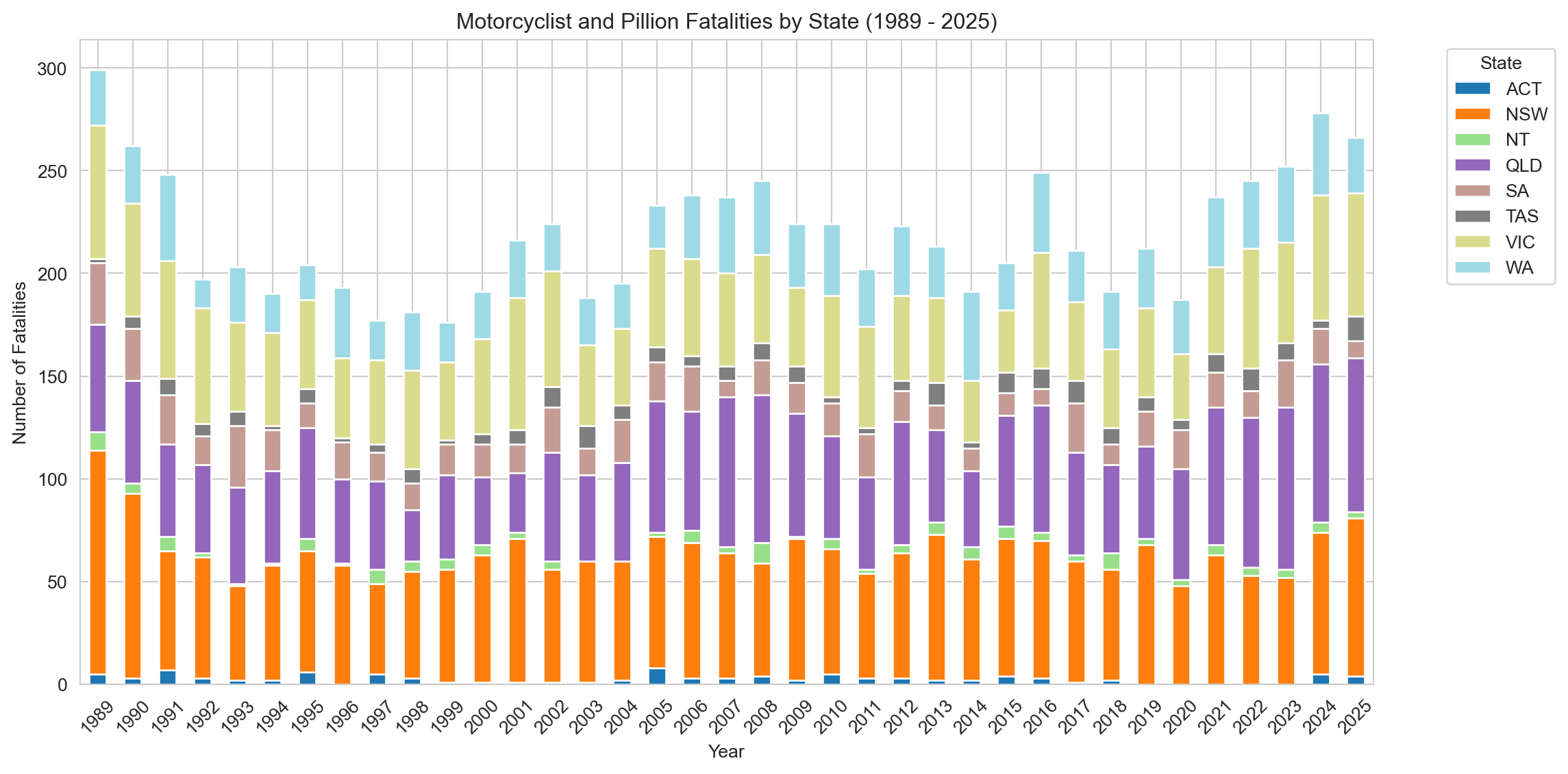
# Group data by Year and State
fatalities_by_year_state = motorcyclist_pillion_fatalities.groupby(['Year', 'State'])['Crash ID'].count().reset_index(name='Fatalities')

# Create a pivot table for the stacked bar chart
pivot_fatalities_state = fatalities_by_year_state.pivot(index='Year', columns='State', values='Fatalities').fillna(0)

# Sort the index to make sure years are in order
pivot_fatalities_state = pivot_fatalities_state.sort_index()

# Plotting stacked bar chart
sns.set_style('whitegrid')
pivot_fatalities_state.plot(kind='bar', stacked=True, figsize=(12, 6), cmap='tab20') # Using a colormap suitable for categorical data
plt.title(f'Motorcyclist and Pillion Fatalities by State ({earliest_year} - {latest_year})')
plt.xlabel('Year')
plt.ylabel('Number of Fatalities')
plt.legend(title='State', bbox_to_anchor=(1.05, 1), loc='upper left') # Adjust legend position
plt.xticks(rotation=45)
plt.tight_layout()
plt.show()

The distribution of fatalities largely mirrors population size and urbanisation, with NSW, Queensland, Victoria, and Western Australia accounting for the bulk of cases across the dataset. This is broadly expected — these states contain the largest populations and the greatest total road networks. However, population alone doesn’t tell the full story. States like Queensland and Western Australia have vast rural and outback road systems where emergency response times are longer, roads are less forgiving, and fatalities are less likely to be prevented by timely medical intervention. The Northern Territory, despite its small population, has historically recorded disproportionately high road fatality rates overall — and this pattern likely extends to motorcyclists, though raw counts may appear modest.It is also worth noting that the stacked bar chart reflects absolute counts rather than rates, which limits direct comparison between states. A per-capita or per-licensed-rider view would likely surface meaningful differences — particularly for smaller jurisdictions. Nonetheless, the chart provides a useful long-run picture of how each state has contributed to the national toll, and whether any state shows a structural shift over time.

3.3 Age Distribution

Code

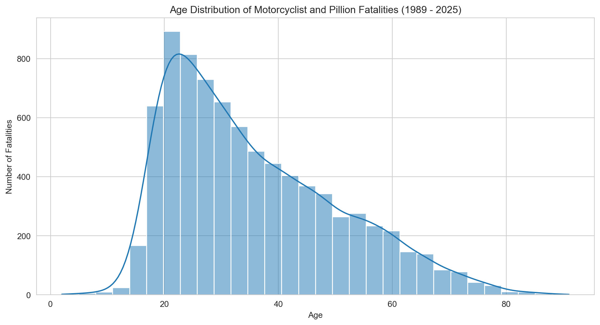
# Plotting the age distribution for motorcyclists and pillion passengers
sns.set_style('whitegrid')
plt.figure(figsize=(12, 6))
sns.histplot(motorcyclist_pillion_fatalities['Age'].dropna(), bins=30, kde=True) # Drop NA values for plotting
plt.title(f'Age Distribution of Motorcyclist and Pillion Fatalities ({earliest_year} - {latest_year})')
plt.xlabel('Age')
plt.ylabel('Number of Fatalities')
plt.grid(True)
plt.show()

Fatalities peak sharply among riders in their early-to-mid 20s, before tapering off through middle age and declining steeply beyond 60. This age profile is consistent with broader road fatality trends — younger riders tend to be newer to the road, more likely to take risks, and statistically over-represented in crashes across all vehicle types. For motorcyclists specifically, inexperience is compounded by the unforgiving nature of two-wheeled travel: there is no crumple zone, no airbag, and little margin for error at speed.The gradual decline after the mid-20s peak likely reflects a combination of improved skill with experience, lifestyle changes that reduce riding frequency, and a natural attrition of higher-risk riders from the road. That said, the distribution does not fall to zero with age — a meaningful tail persists into the 50s and 60s, reflecting the growing cohort of older recreational riders who return to or remain on motorcycles in retirement. This group presents a different risk profile: while they may ride more cautiously, older riders are physiologically more vulnerable to crash injury, and their fatalities may be more likely to result from medical complications than pure crash severity. The data suggests that no single age group can be considered low-risk when it comes to motorcycling.

3.4 Gender Breakdown

Code

# Filter out missing gender values
gender_fatalities = motorcyclist_pillion_fatalities.dropna(subset=['Gender'])

# Group data by Gender, counting all Crash ID occurrences
gender_count = gender_fatalities.groupby('Gender')['Crash ID'].count().reset_index(name='Fatalities')

# Plotting a bar plot for Gender breakdown
plt.figure(figsize=(8, 6))
sns.barplot(x='Gender', y='Fatalities', data=gender_count, hue='Gender', palette=custom_palette, dodge=False, legend=False)
plt.title(f'Motorcyclist and Pillion Fatalities by Gender ({earliest_year} - {latest_year})') 
plt.xlabel('Gender')
plt.ylabel('Number of Fatalities')
plt.tight_layout()
plt.show()

# # Calculate and print the percentage
# gender_count['Percentage'] = (gender_count['Fatalities'] / gender_count['Fatalities'].sum()) * 100
# print("Gender Breakdown (%):")
# print(gender_count[['Gender', 'Percentage']])

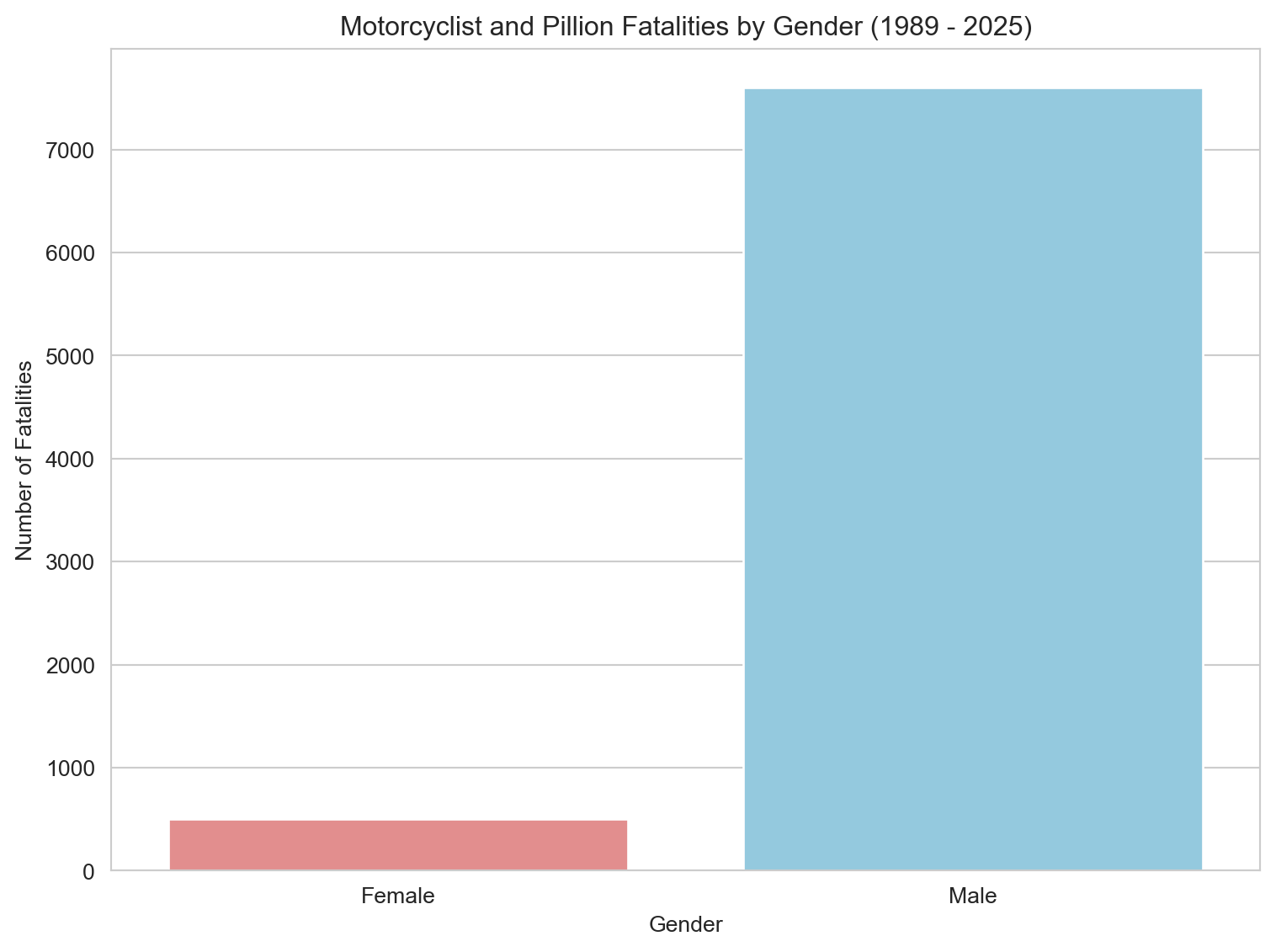
Male riders accounted for 93.7% of all fatalities — a stark imbalance that reflects both who rides and how they ride. While far more men hold motorcycle licenses, the gap is also driven by risk-taking behaviour: younger male riders are more prone to speeding, aggressive cornering, and risky overtaking. The gender disparity is not just about exposure — it’s also about the choices made on the road.

Code

# Ratio of gender fatalities of pillion passengers

# Filter out missing gender values for pillion passengers
pillion_gender_fatalities = pillion_fatalities.dropna(subset=['Gender'])

# Group data by Gender, counting all Crash ID occurrences for pillions
pillion_gender_count = pillion_gender_fatalities.groupby('Gender')['Crash ID'].count().reset_index(name='Fatalities')

# Calculate percentages
pillion_gender_count['Percentage'] = (pillion_gender_count['Fatalities'] / pillion_gender_count['Fatalities'].sum()) * 100

# Print the percentages
print("Pillion Passenger Gender Breakdown (%):")
print(pillion_gender_count[['Gender', 'Percentage']])

# Plotting a bar plot for Pillion Gender breakdown percentages
plt.figure(figsize=(8, 6))
sns.barplot(x='Gender', y='Percentage', data=pillion_gender_count, hue='Gender', palette=custom_palette, dodge=False, legend=False)
plt.title(f'Pillion Passenger Fatalities by Gender (%) ({earliest_year} - {latest_year})')
plt.xlabel('Gender')
plt.ylabel('Percentage of Pillion Fatalities (%)')
plt.ylim(0, 100) # Set y-axis limit to 100%
plt.tight_layout()
plt.show()

# Note to self: future expansion on pillion passenger risks
# - Consider expanding on the gender imbalance in pillion passenger fatalities (56% female vs 44% male).
# - Explore cultural and behavioural explanations — e.g. women more likely to ride as passengers than operate motorcycles.
# - Investigate risk differences for pillions: seating position, lack of protective gear, and limited control.
# - Possibly link to public health campaigns (or lack thereof) targeting pillion safety.
# - Could include qualitative anecdotes or policy gaps for supporting data storytelling.

Pillion Passenger Gender Breakdown (%):
   Gender  Percentage
0  Female   55.754476
1    Male   44.245524

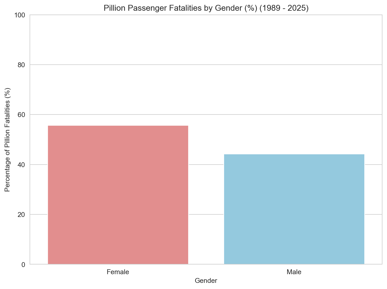
Pillion passenger fatalities show a gendered pattern, with 56% of deaths involving female passengers and 44% male. This stands in contrast to rider fatalities, which are overwhelmingly male. The data reflects broader social dynamics — women are more likely to be passengers than riders, and pillion safety is rarely given the same attention in safety campaigns or gear design.

Code

# Filter out missing Age or Gender values for the plot
age_gender_data = motorcyclist_pillion_fatalities.dropna(subset=['Age', 'Gender'])

# Plotting the violin plot
plt.figure(figsize=(10, 7))
sns.violinplot(x='Gender', y='Age', data=age_gender_data, palette=custom_palette, hue='Gender', legend=False)
plt.title(f'Age Distribution of Motorcyclist and Pillion Fatalities by Gender ({earliest_year} - {latest_year})')
plt.xlabel('Gender')
plt.ylabel('Age')
plt.yticks(np.arange(0, 101, 10)) # Set y-ticks from 0 to 100
plt.grid(axis='y', linestyle='--', alpha=0.7)
plt.show()

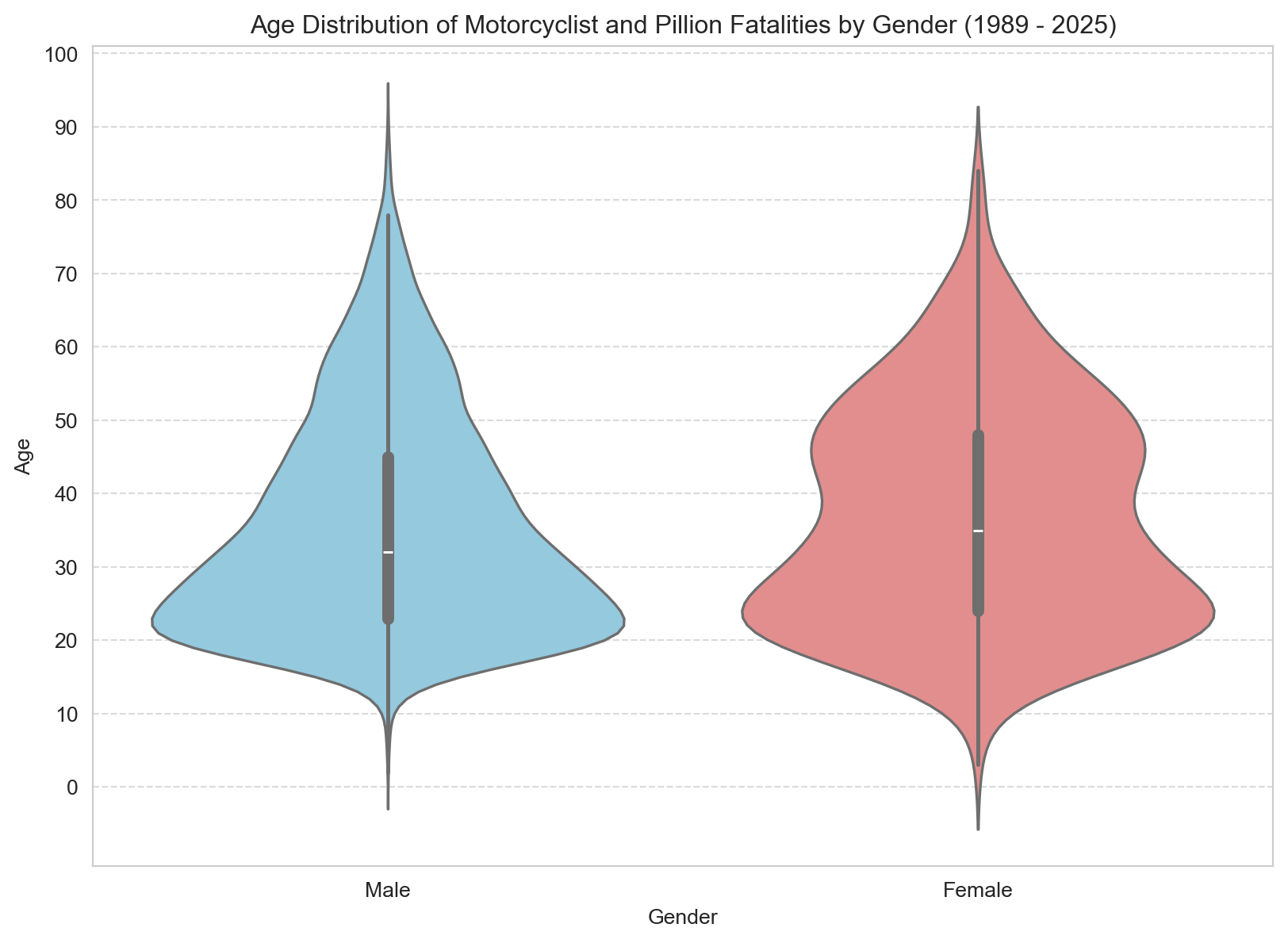
Male fatalities cluster sharply in the 20s and 30s, consistent with the overall age histogram. Female fatalities, while far fewer, show a slightly broader and older distribution — with a possible double peak hinting at two cohorts: younger pillions and older recreational riders. The sample is small, so caution is warranted, but the pattern suggests that female riders and passengers involved in fatal crashes tend to be somewhat older than their male counterparts.

3.5 Monthly Trends

Code

# Map month numbers to names
month_counts_df = motorcyclist_pillion_fatalities.copy() # Use copy to avoid SettingWithCopyWarning if modifying view
month_counts_df['Month Name'] = month_counts_df['Month'].map(month_names)

# Calculate the number of fatalities by month
month_counts = month_counts_df['Month Name'].value_counts().reset_index()
month_counts.columns = ['Month', 'Fatalities']

# Sort the months in calendar order
month_counts['Month'] = pd.Categorical(month_counts['Month'], categories=month_order, ordered=True)
month_counts = month_counts.sort_values('Month')

# Plotting a bar plot for monthly breakdown
plt.figure(figsize=(12, 6))
sns.barplot(x='Month', y='Fatalities', data=month_counts, hue='Month', palette='viridis', dodge=False, legend=False) # Changed palette
plt.title(f'Motorcyclist and Pillion Fatalities by Month ({earliest_year} - {latest_year})')
plt.xlabel('Month')
plt.ylabel('Number of Fatalities')
plt.xticks(rotation=45)
plt.tight_layout()
plt.show()

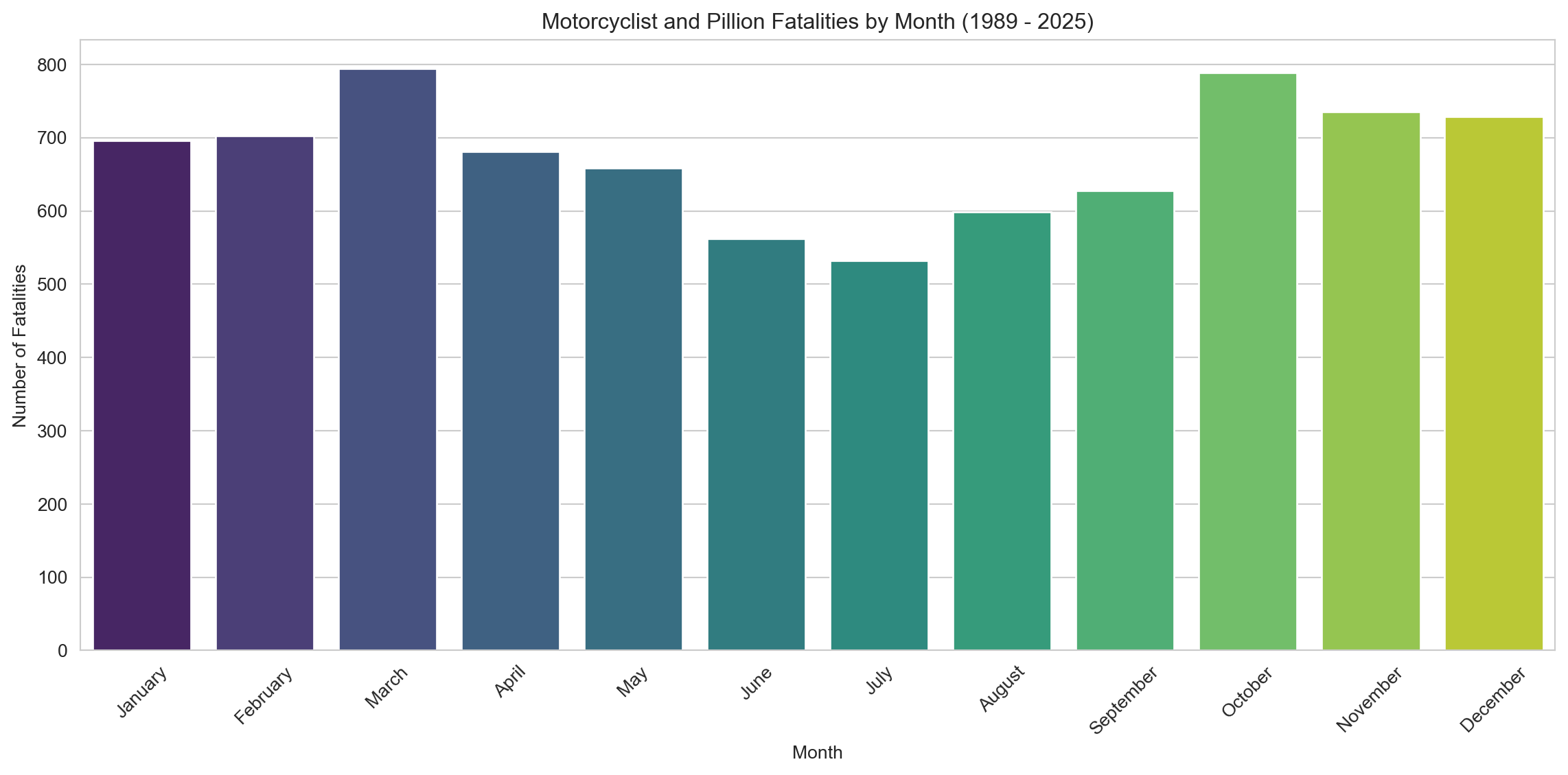
Winter records the fewest fatalities — June and July in particular, when cold and wet conditions keep many bikes parked. Fatalities peak during the warmer months, especially March, October, and November, when riding conditions are ideal and recreational activity spikes.

3.6 Time of Day vs Day of Week

Code

# Select relevant columns and drop missing Time values
heatmap_df = motorcyclist_pillion_fatalities[['Time', 'Dayweek']].dropna(subset=['Time']).copy()

# Extracting the hour from the time field
heatmap_df['Hour'] = heatmap_df['Time'].str.split(':').str[0].astype(int)

# Creating a pivot table
pivot_table = pd.pivot_table(heatmap_df,
                            values='Time',
                            index=['Hour'],
                            columns=['Dayweek'],
                            aggfunc='count',
                            fill_value=0)

# Reindex to ensure all hours and days are present and ordered correctly
pivot_table = pivot_table.reindex(range(24), fill_value=0)
pivot_table = pivot_table.reindex(columns=day_order, fill_value=0) # Use the predefined day_order

# Plotting the heatmap
plt.figure(figsize=(12, 8))
sns.heatmap(pivot_table, 
            annot=True, 
            cmap='RdYlGn_r', # Reversed Red-Yellow-Green colormap
            fmt='g') # General format for annotations
plt.title(f'Motorcyclist and Pillion Fatalities by Day of Week and Hour of Day ({earliest_year} - {latest_year})')
plt.xlabel('Day of the Week')
plt.ylabel('Hour of Day')
plt.show()

# # Note to self: Do two further plots

# Weekday crashes might skew toward multi-vehicle, likely tied to commuting hours — think lane filtering gone wrong, inattentive drivers during peak traffic, or intersections in city zones.

# Weekend crashes, on the other hand, might lean heavily toward single-vehicle incidents, especially on winding, high-speed rural roads (the twisties). This would back the theory that rider error, overconfidence, or unfamiliarity with terrain plays a major role.

The most dangerous time to ride is Saturday and Sunday afternoon — fatalities concentrate sharply between 11am and 4pm on weekends. The pattern points clearly to recreational riding: less frequent riders on unfamiliar or technical roads, often pushing harder than their skill level warrants. Weekday fatalities are more evenly spread across the day and likely reflect a different risk profile — commuters navigating traffic in urban environments.

3.7 Single vs Multi-Vehicle Crashes

Code

# Calculate counts for each Crash Type
crash_type_counts = motorcyclist_pillion_fatalities['Crash Type'].value_counts().reset_index()
crash_type_counts.columns = ['Crash Type', 'Fatalities']

# Calculate percentages
crash_type_counts['Percentage'] = (crash_type_counts['Fatalities'] / crash_type_counts['Fatalities'].sum()) * 100

# Print the percentages
print("Crash Type Breakdown (%):")
print(crash_type_counts[['Crash Type', 'Percentage']])

# Plotting the bar chart of percentages
plt.figure(figsize=(8, 6))
sns.barplot(x='Crash Type', y='Percentage', data=crash_type_counts, hue='Crash Type', palette='coolwarm', dodge=False, legend=False)
plt.title(f'Percentage of Single vs Multi-Vehicle Crashes ({earliest_year} - {latest_year})')
plt.xlabel('Crash Type')
plt.ylabel('Percentage of Fatalities (%)')
plt.ylim(0, 100) # Set y-axis limit to 100%
plt.tight_layout()
plt.show()

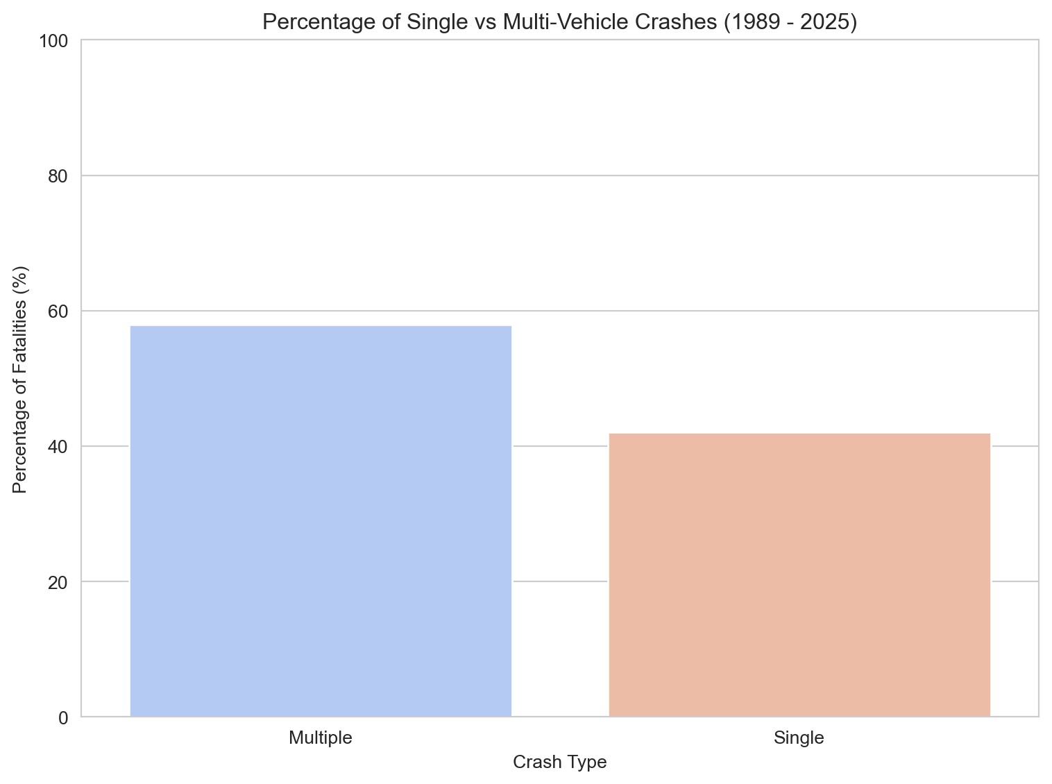
Crash Type Breakdown (%):
  Crash Type  Percentage
0   Multiple   57.962255
1     Single   42.037745

Analysis of crash types from 1989 to 2021 reveals that 58% of fatal motorcycle crashes involved another vehicle, while 42% were single-vehicle incidents. This finding highlights that a significant portion of fatalities occur without another party involved, suggesting that rider behavior, decision-making, or road conditions may play an important role.

The high proportion of single-vehicle motorcycle fatalities reinforces a longstanding principle in motorcycle safety: the rider themselves is often the greatest risk factor. While not all single-vehicle crashes stem from rider error, the data implies that many of these tragic events could potentially be mitigated through improved rider training, safer riding practices, and hazard awareness. It also raises questions about infrastructure and road maintenance, both of which disproportionately affect motorcyclists.

In contrast, multi-vehicle crashes remind us that vigilance is equally required around other road users, many of whom may fail to detect or respect motorcyclists. Together, these figures point to the need for both personal responsibility and broader systemic efforts to protect motorcyclists.

Code

# Line Graph of Proportions Over Time

# Group by Year and Crash Type, count fatalities
fatalities_by_year_crash_type = motorcyclist_pillion_fatalities.groupby(['Year', 'Crash Type'])['Crash ID'].count().reset_index(name='Fatalities')

# Calculate total fatalities per year
total_fatalities_per_year = fatalities_by_year_crash_type.groupby('Year')['Fatalities'].transform('sum')

# Calculate proportion for each crash type per year
fatalities_by_year_crash_type['Proportion'] = (fatalities_by_year_crash_type['Fatalities'] / total_fatalities_per_year) * 100

# Plotting the line graph of proportions
plt.figure(figsize=(12, 6))
sns.lineplot(x='Year', 
            y='Proportion', 
            data=fatalities_by_year_crash_type, 
            hue='Crash Type', 
            marker='o',
            palette='coolwarm')
plt.title(f'Proportion of Single vs Multi-Vehicle Crashes Over Time ({earliest_year} - {latest_year})')
plt.xlabel('Year')
plt.ylabel('Proportion of Fatalities (%)')
plt.ylim(0, 100) # Set y-axis limit to 100%
plt.grid(True)
sns.despine()
plt.legend(title='Crash Type')
plt.tight_layout()
plt.show()

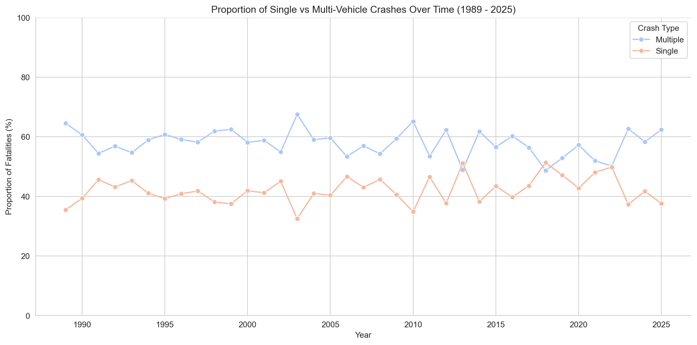
Analysis of fatal motorcycle crashes by type reveals an emerging trend: since 2015, the proportion of single-vehicle fatalities has been gradually increasing, while multi-vehicle fatalities have declined — a convergence not seen in earlier decades. This is especially noteworthy given the context of major technological and safety advancements in motorcycling during this period.

Modern motorcycles, including mid-range performance bikes, now come equipped with advanced safety features such as traction control, ABS, multiple rider modes, wheelie control, and quickshifters. High-end models even offer lean-angle-sensitive ABS, cornering lights, and ride-by-wire throttles. Simultaneously, protective gear has improved dramatically — with the rise of ECE 22.06-certified helmets, airbag vests, and CE Level 2-rated armor becoming increasingly standard and affordable.

Despite these improvements, the relative rise in single-vehicle fatalities suggests that technology alone is not enough to prevent crashes. These incidents may stem from factors like excessive speed, rider inexperience, or misjudgment on corners and rural roads — scenarios where rider behavior and decision-making remain the dominant risk factors. It reinforces the idea that while safety features can mitigate outcomes, they cannot eliminate the inherent risk of riding. This underscores the ongoing need for rider education, road awareness, and perhaps cultural shifts within the motorcycling community toward valuing defensive riding as much as performance and thrill.

Code

# Step 1: Compute proportions
day_crash_prop = (
    motorcyclist_pillion_fatalities
    .groupby(['Day of week', 'Crash Type'])['Crash ID']
    .count()
    .unstack() # Pivot 'Crash Type' to columns
    .apply(lambda x: x / x.sum(), axis=1) # Calculate proportion across columns (within each 'Day of week')
    .stack() # Convert back to long format
    .rename("Proportion")
    .reset_index()
)

# Step 2: Plot
sns.set_style("whitegrid")
plt.figure(figsize=(8, 5))
sns.barplot(data=day_crash_prop, x='Day of week', y='Proportion', hue='Crash Type')
plt.title('Proportion of Motorcycle Fatalities: Single vs Multiple Vehicle Crashes\nBy Weekday vs Weekend')
plt.ylabel('Proportion')
plt.xlabel('')
plt.ylim(0, 1)
plt.legend(title='Crash Type')
plt.tight_layout()
plt.show()

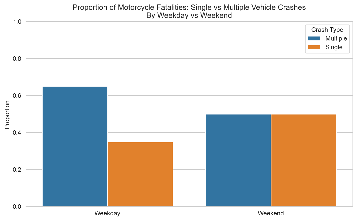
On weekdays, a greater proportion of fatal crashes involve multiple vehicles — consistent with commuter conditions and interactions with other road users. On weekends the pattern inverts: single-vehicle crashes edge ahead of multi-vehicle ones, reinforcing the picture of recreational riders losing control on open roads rather than colliding with other traffic. Effective interventions look quite different depending on when and why people ride.

4. Conclusion

Motorcyclists remain one of the highest-risk groups on Australian roads. Across three decades of data, the same pattern appears repeatedly: fatalities concentrate on weekends, during daylight hours, and among younger male riders.

Normalising by licence counts shows that risk has not fallen in a clear, sustained way over the period where licence data is available. That suggests broad road safety gains have not translated cleanly to motorcyclists.

Future work could explore: - Crash severity by motorcycle type or engine capacity - Weather and road-condition effects - Post-licensure experience (for example, L/P plate history where available)

Overall, the findings support targeted interventions for loss-of-control crashes, especially in weekend recreational riding contexts.