---
title: "{{< var study_title >}}"
subtitle: "Exploratory Data Analysis"
---
## Setup
```{r}
#| label: setup
#| collapse: true
#| code-summary: "Load packages and helpers"
library(here)
library(tidyverse)
library(arrow)
library(gtsummary)
library(janitor)

source(here("R", "utils.R"))       # miss_summary(), fmt_pval(), n_pct(), etc.
source(here("R", "plot_theme.R"))  # theme_epi(), scale_fill_epi(), save_fig()
```
`tidyverse` covers data wrangling and visualisation; `arrow` reads the Parquet file produced by the SQL pipeline; `gtsummary` generates publication-ready Table 1s and univariable regression summaries. Project-level helpers are sourced from `R/`.
---
## Data Pipeline
The raw BRFSS 2024 data were downloaded as a SAS XPT file and converted to Parquet using `R/xpt_to_parquet.R`. The mart was built using DuckDB with four SQL scripts run in sequence: a view over the raw Parquet file, a recode and inclusion-criteria step to produce the analytical dataset, validation checks, and export to Parquet for use in R.
```{sql}
--| label: sql-load-raw
--| code-summary: "01: Create view over raw Parquet file"
--| eval: false
-- 01_load_raw.sql
-- Create a view over the raw Parquet file so DuckDB can query it by name.
create or replace view brfss_raw as
select * from read_parquet('data/raw/LLCP2024.parquet');

select count(*) as n_rows from brfss_raw;
```
```{sql}
--| label: sql-build-mart
--| code-summary: "02: Recode variables and apply inclusion criteria"
--| eval: false
-- 02_build_mart.sql
-- Select and recode all variables, then filter to respondents with a
-- non-missing diabetes outcome (DIABETE4 codes 7, 9, and 2 set to NULL).
create or replace table analytical_dataset as
with base as (
    select
        -- Survey design variables (retained for potential weighted analysis)
        _PSU as psu,
        _STSTR as strata,
        _LLCPWT as llcp_weight,
        -- Raw outcome variable
        DIABETE4 as diabetes_raw,
        -- Demographic predictors
        _AGEG5YR as age_group_raw,
        SEXVAR as sex_raw,
        _RACE as race_raw,
        -- Social determinants
        _EDUCAG as education_raw,
        _INCOMG1 as income_raw,
        PERSDOC3 as has_provider_raw,
        -- Clinical / behavioural predictors
        _BMI5CAT as bmi_cat_raw,
        _TOTINDA as phys_activity_raw,
        _SMOKER3 as smoking_raw,
        _RFDRHV9 as heavy_alcohol_raw,
        _MENT14D as mental_health_raw
    FROM brfss_raw
),

recoded as (
    select
        psu,
        strata,
        llcp_weight,
        case
            when diabetes_raw = 1 then 1
            when diabetes_raw in (3, 4) then 0
            else null -- 2, 7, 9 are various forms of missingness
        end as diabetes,
        case
            when age_group_raw in (1, 2) then '18-34'
            when age_group_raw in (3, 4) then '35-44'
            when age_group_raw in (5, 6) then '45-54'
            when age_group_raw in (7, 8) then '55-64'
            when age_group_raw in (9, 10) then '65-74'
            when age_group_raw in (11, 12, 13) then '75+'
            else null
        end as age_group,
        case
            when sex_raw = 1 then 'Male'
            when sex_raw = 2 then 'Female'
            else null
        end as sex,
        -- Race/ethnicity: CDC combines race and Hispanic ethnicity into a single
        -- computed variable. Hispanic is its own category regardless of race.
        -- NH (Non-Hispanic) prefix is dropped for clarity for non-US readers.
        case
            when race_raw = 1 then 'White'
            when race_raw = 2 then 'Black'
            when race_raw = 3 then 'American Indian/Alaskan Native'
            when race_raw = 4 then 'Asian'
            when race_raw = 5 then 'Pacific Islander'
            when race_raw = 6 then 'Other/Multiracial'
            when race_raw = 7 then 'Hispanic'
            when race_raw = 8 then 'Other'
            else null
        end as race_ethnicity,
        case
            when education_raw = 1 then 'Did not graduate high school'
            when education_raw = 2 then 'High school graduate'
            when education_raw = 3 then 'Some college'
            when education_raw = 4 then 'College graduate'
            else null
        end as education,
        case
            when income_raw = 1 then '<$15k'
            when income_raw = 2 then '$15k-$25k'
            when income_raw = 3 then '$25k-$35k'
            when income_raw = 4 then '$35k-$50k'
            when income_raw = 5 then '$50k-$100k'
            when income_raw = 6 then '>$100k'
            else null
        end as income_group,
        case
            when has_provider_raw in (1, 2) then 1
            when has_provider_raw = 3 then 0
            else null
        end as has_provider,
        case
            when bmi_cat_raw = 1 then 'Underweight'
            when bmi_cat_raw = 2 then 'Normal'
            when bmi_cat_raw = 3 then 'Overweight'
            when bmi_cat_raw = 4 then 'Obese'
            else null
        end as bmi_category,
        case
            when phys_activity_raw = 1 then 1
            when phys_activity_raw = 2 then 0
            else null
        end as physically_active,
        case
            when smoking_raw = 1 then 'Current (daily)'
            when smoking_raw = 2 then 'Current (some days)'
            when smoking_raw = 3 then 'Former'
            when smoking_raw = 4 then 'Never'
            else null
        end as smoking_status,
        case
            when heavy_alcohol_raw = 1 then 0
            when heavy_alcohol_raw = 2 then 1
            else null
        end as heavy_drinker,
        case
            when mental_health_raw = 1 then '0 days'
            when mental_health_raw = 2 then '1-13 days'
            when mental_health_raw = 3 then '14+ days'
            else null
        end as mental_health_days
    from base
)
select * from recoded
where diabetes is not null;
```
```{sql}
--| label: sql-validation
--| code-summary: "03: Validation checks"
--| eval: false
-- 03_validation.sql
-- Row counts, outcome distribution, and missingness by predictor.
select count(*) from analytical_dataset;

select
    diabetes,
    count(*) as n,
    round(100.0 * count(*) / sum(count(*)) over (), 2) as pct
from analytical_dataset
group by diabetes
order by diabetes;

select
    count(*) filter (where age_group is null) as miss_age,
    count(*) filter (where sex is null) as miss_sex,
    count(*) filter (where race_ethnicity is null) as miss_race,
    count(*) filter (where education is null) as miss_education,
    count(*) filter (where income_group is null) as miss_income,
    count(*) filter (where bmi_category is null) as miss_bmi,
    count(*) filter (where physically_active is null) as miss_activity,
    count(*) filter (where smoking_status is null) as miss_smoking,
    count(*) filter (where heavy_drinker is null) as miss_alcohol,
    count(*) filter (where has_provider is null) as miss_provider,
    count(*) filter (where mental_health_days is null) as miss_mh
from analytical_dataset;

select bmi_category, diabetes, count(*) as n
from analytical_dataset
where bmi_category is not null
group by bmi_category, diabetes
order by bmi_category, diabetes;
```
```{sql}
--| label: sql-export
--| code-summary: "04: Export to Parquet"
--| eval: false
-- 04_export.sql
copy (select * from analytical_dataset)
to 'data/processed/analysis_dataset.parquet'
(format parquet);
```
The Parquet file is the mart for analysis: the raw data file stays untouched, and all downstream R code reads from `data/processed/`.
---
## Data Import
```{r}
#| label: import
#| collapse: true
df <- read_parquet(here("data", "processed", "analysis_dataset.parquet"))
dim(df)
names(df)
```
The analytical dataset contains `r nrow(df)` respondents with a fully observed binary outcome; rows with missing or ambiguous diabetes responses (codes 2, 7, 9 in `DIABETE4`) were removed during the SQL build step. The columns include three survey design fields (`psu`, `strata`, `llcp_weight`) and `r ncol(df) - 4` demographic, socioeconomic, and behavioural predictors. No further outcome filtering is needed, so any remaining issues lie in predictor encoding and missingness.
---
## Sample Characteristics
### Predictor distributions
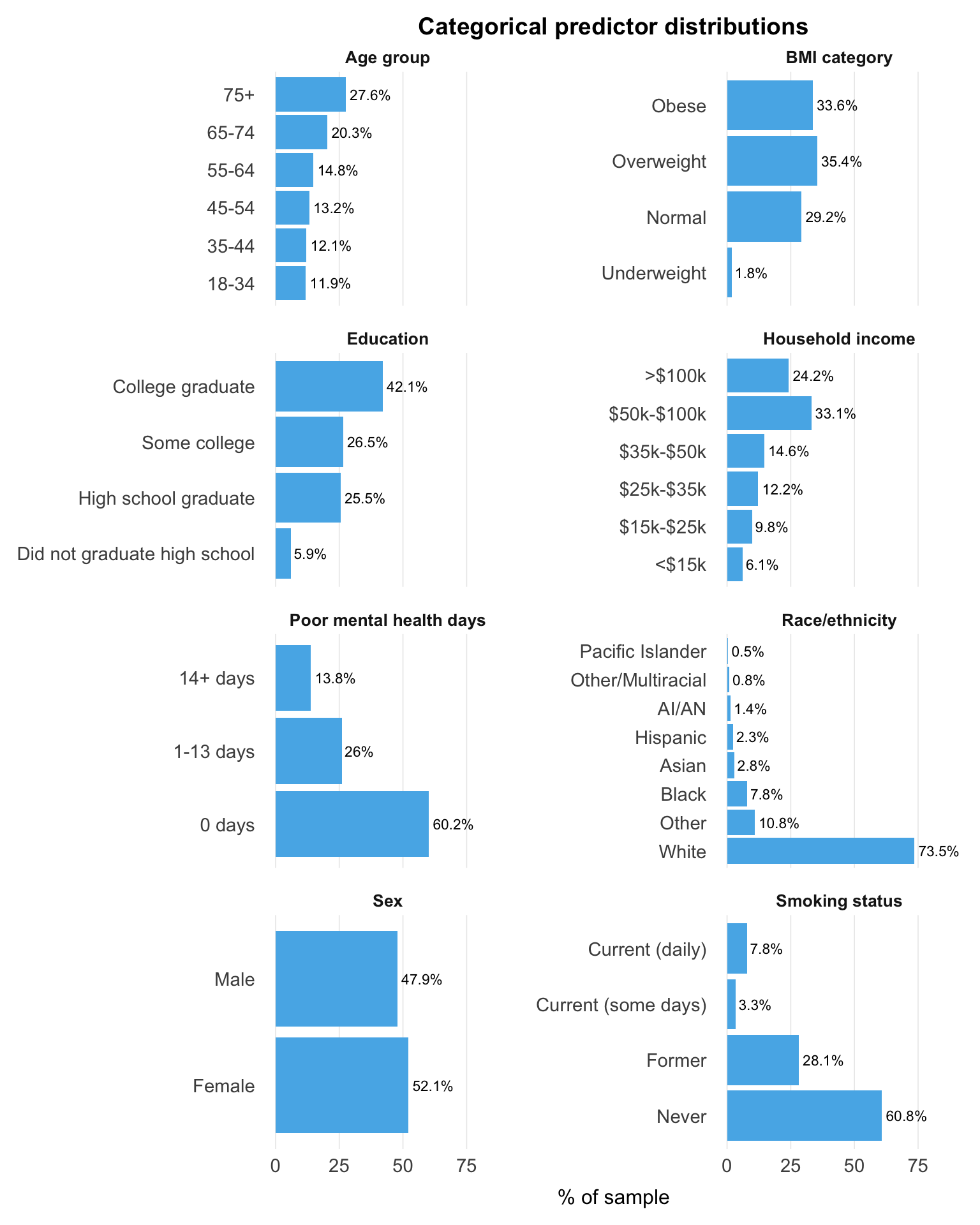
Understanding the sample composition across predictors helps identify sparse categories, where estimates will be less stable.
```{r}
#| label: predictor-distributions
#| fig-cap: "Categorical predictor distributions"
#| fig-height: 10
df_dist <- df |>
  mutate(
    age_group          = factor(age_group,
                                levels = c("18-34", "35-44", "45-54", "55-64", "65-74", "75+")),
    education          = factor(education,
                                levels = c("Did not graduate high school", "High school graduate",
                                           "Some college", "College graduate")),
    income_group       = factor(income_group,
                                levels = c("<$15k", "$15k-$25k", "$25k-$35k",
                                           "$35k-$50k", "$50k-$100k", ">$100k")),
    bmi_category       = factor(bmi_category,
                                levels = c("Underweight", "Normal", "Overweight", "Obese")),
    smoking_status     = factor(smoking_status,
                                levels = c("Never", "Former",
                                           "Current (some days)", "Current (daily)")),
    mental_health_days = factor(mental_health_days,
                                levels = c("0 days", "1-13 days", "14+ days"))
  )

cat_vars <- c("age_group", "sex", "race_ethnicity", "education", "income_group",
              "bmi_category", "smoking_status", "mental_health_days")

dist_data <- purrr::map_dfr(cat_vars, function(v) {
  counts <- df_dist |>
    filter(!is.na(.data[[v]])) |>
    count(variable = v, level = as.character(.data[[v]])) |>
    mutate(pct = n / sum(n) * 100)

  if (is.factor(df_dist[[v]])) {
    counts |> mutate(level = factor(level, levels = levels(df_dist[[v]])))
  } else {
    counts |> arrange(desc(n)) |> mutate(level = factor(level, levels = unique(level)))
  }
}) |>
  mutate(level = fct_recode(level,
                             "AI/AN" = "American Indian/Alaskan Native"))

facet_labels <- c(
  age_group          = "Age group",
  sex                = "Sex",
  race_ethnicity     = "Race/ethnicity",
  education          = "Education",
  income_group       = "Household income",
  bmi_category       = "BMI category",
  smoking_status     = "Smoking status",
  mental_health_days = "Poor mental health days"
)

ggplot(dist_data, aes(x = pct, y = level)) +
  geom_col(fill = palette_epi[["sky_blue"]], show.legend = FALSE) +
  geom_text(aes(label = paste0(round(pct, 1), "%")), hjust = -0.1, size = 3) +
  facet_wrap(~variable, scales = "free_y", ncol = 2,
             labeller = as_labeller(facet_labels)) +
  labs(x = "% of sample", y = NULL,
       title = "Categorical predictor distributions") +
  xlim(0, max(dist_data$pct) * 1.2) +
  theme(
    panel.grid.major.y = element_blank(),
    panel.grid.minor   = element_blank(),
    panel.grid.major.x = element_line(colour = "grey92", linewidth = 0.3),
    plot.title         = element_text(hjust = 0.5, size = 14, face = "bold"),
    strip.text         = element_text(face = "bold", size = 10)
  )
```
The sample skews older and more educated: adults aged 65 and over make up 48% of respondents, and college graduates are the largest education category (42.1%). Most respondents (69%) are overweight or obese, so BMI contrasts are well represented in the data. The most consequential imbalance is in race and ethnicity. White respondents account for 73.5% of the sample, while several groups (Pacific Islander, American Indian or Alaska Native, Other/Multiracial, Hispanic, and Asian) each fall below 3%, so their estimates will be less precise and need cautious interpretation.
```{r}
#| label: binary-predictors
#| fig-cap: "Binary predictor prevalence"
#| fig-height: 3
binary_labels <- c(
  physically_active = "Physically active",
  heavy_drinker     = "Heavy drinker",
  has_provider      = "Has personal doctor"
)

binary_data <- tibble(
  variable = names(binary_labels),
  label    = binary_labels
) |>
  mutate(pct = map_dbl(variable, ~mean(df[[.x]], na.rm = TRUE) * 100)) |>
  arrange(pct) |>
  mutate(label = factor(label, levels = label))

ggplot(binary_data, aes(x = pct, y = label)) +
  geom_segment(aes(x = 0, xend = pct, yend = label),
               colour = palette_epi[["sky_blue"]]) +
  geom_point(colour = palette_epi[["sky_blue"]], size = 3) +
  geom_text(aes(label = paste0(round(pct, 1), "%")),
            hjust = -0.3, size = 3) +
  labs(x = "% of sample", y = NULL,
       title = "Binary predictor prevalence") +
  xlim(0, 105) +
  theme(
    panel.grid.major.y = element_blank(),
    panel.grid.minor   = element_blank(),
    panel.grid.major.x = element_line(colour = "grey92", linewidth = 0.3),
    plot.title         = element_text(hjust = 0.5, size = 14, face = "bold")
  )
```
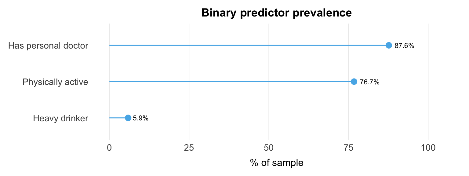
All three binary predictors are strongly imbalanced. Heavy drinking is rare (5.9%), so estimates of its association with diabetes rest on a small exposed group. Having a personal doctor (87.6%) and being physically active (76.7%) are also one-sided, which limits contrast and precision.
### Outcome prevalence
```{r}
#| label: outcome-prevalence
#| collapse: true
prev <- df |>
  count(diabetes) |>
  mutate(
    prop = n / sum(n),
    pct  = scales::percent(prop, accuracy = 0.1)
  )

prev
```
`r prev$pct[prev$diabetes == 1]` of respondents (`r format(prev$n[prev$diabetes == 1], big.mark = ",")` of `r format(sum(prev$n), big.mark = ",")`) reported a diabetes diagnosis. The outcome is moderately imbalanced rather than rare: there are enough cases for stable estimation, but the imbalance matters when interpreting results.
### Table 1: Sample characteristics by diabetes status
```{r}
#| label: table-one
df |>
  select(
    diabetes,
    age_group, sex, race_ethnicity, education, income_group,
    bmi_category, physically_active, smoking_status,
    heavy_drinker, has_provider, mental_health_days
  ) |>
  mutate(
    diabetes   = factor(diabetes, levels = c(0, 1), labels = c("No diabetes", "Diabetes")),
    age_group  = factor(age_group,
                        levels = c("18-34", "35-44", "45-54", "55-64", "65-74", "75+")),
    education  = factor(education,
                        levels = c("Did not graduate high school", "High school graduate",
                                   "Some college", "College graduate")),
    income_group = factor(income_group,
                          levels = c("<$15k", "$15k-$25k", "$25k-$35k",
                                     "$35k-$50k", "$50k-$100k", ">$100k")),
    bmi_category = factor(bmi_category,
                          levels = c("Underweight", "Normal", "Overweight", "Obese")),
    smoking_status = factor(smoking_status,
                            levels = c("Never", "Former", "Current (some days)", "Current (daily)"))
  ) |>
  tbl_summary(
    by      = diabetes,
    missing = "no",
    label   = list(
      age_group          ~ "Age group",
      sex                ~ "Sex",
      race_ethnicity     ~ "Race/ethnicity",
      education          ~ "Education",
      income_group       ~ "Household income",
      bmi_category       ~ "BMI category",
      physically_active  ~ "Physically active",
      smoking_status     ~ "Smoking status",
      heavy_drinker      ~ "Heavy drinker",
      has_provider       ~ "Has personal doctor",
      mental_health_days ~ "Poor mental health days"
    )
  ) |>
  add_p() |>
  add_overall() |>
  bold_p(t = 0.05) |>
  bold_labels() |>
  modify_caption("**Table 1.** Sample characteristics by diabetes status")
```
Age and BMI show the strongest gradients: the diabetes group skews substantially older, and obesity is markedly more common (52% vs 30%). Socioeconomic differences follow a similar pattern, with lower income and lower education more prevalent in the diabetes group. Behavioural and health indicators add further contrasts (lower physical activity, more former smokers, and more frequent poor mental health days), though these likely reflect a mix of upstream risk factors and downstream consequences of disease. These overlapping relationships are revisited in the adjusted model.
---
## Outcome Prevalence by Subgroup
```{r}
#| label: prevalence-by-subgroup
#| fig-cap: "Crude diabetes prevalence by key predictor categories"
#| fig-height: 10
df_prev <- df |>
  mutate(smoking_status = factor(smoking_status,
                                  levels = c("Never", "Former",
                                             "Current (some days)", "Current (daily)")))

cat_vars <- c("age_group", "sex", "race_ethnicity", "education",
              "income_group", "bmi_category", "smoking_status",
              "mental_health_days")

facet_labels <- c(
  age_group          = "Age group",
  sex                = "Sex",
  race_ethnicity     = "Race/ethnicity",
  education          = "Education",
  income_group       = "Household income",
  bmi_category       = "BMI category",
  smoking_status     = "Smoking status",
  mental_health_days = "Poor mental health days"
)

prev_data <- purrr::map_dfr(cat_vars, function(v) {
  counts <- df_prev |>
    filter(!is.na(.data[[v]])) |>
    group_by(variable = v, level = .data[[v]]) |>
    summarise(
      n        = n(),
      cases    = sum(diabetes),
      prev_pct = mean(diabetes) * 100,
      .groups  = "drop"
    )

  if (is.factor(df_prev[[v]])) {
    counts |> mutate(level = factor(as.character(level),
                                    levels = levels(df_prev[[v]])))
  } else {
    counts |> arrange(prev_pct) |>
      mutate(level = factor(as.character(level), levels = unique(as.character(level))))
  }
}) |>
  mutate(level = fct_recode(level, "AI/AN" = "American Indian/Alaskan Native"))

ggplot(prev_data, aes(x = prev_pct, y = level)) +
  geom_col(fill = palette_epi[["sky_blue"]], show.legend = FALSE) +
  geom_text(aes(label = paste0(round(prev_pct, 1), "%")),
            hjust = -0.1, size = 3) +
  facet_wrap(~variable, scales = "free_y", ncol = 2,
             labeller = as_labeller(facet_labels)) +
  labs(x = "Diabetes prevalence (%)", y = NULL,
       title = "Crude diabetes prevalence by predictor category") +
  xlim(0, max(prev_data$prev_pct) * 1.2) +
  theme(
    panel.grid.major.y = element_blank(),
    panel.grid.minor   = element_blank(),
    panel.grid.major.x = element_line(colour = "grey92", linewidth = 0.3),
    plot.title         = element_text(hjust = 0.5, size = 14, face = "bold"),
    strip.text         = element_text(face = "bold", size = 10)
  )
```
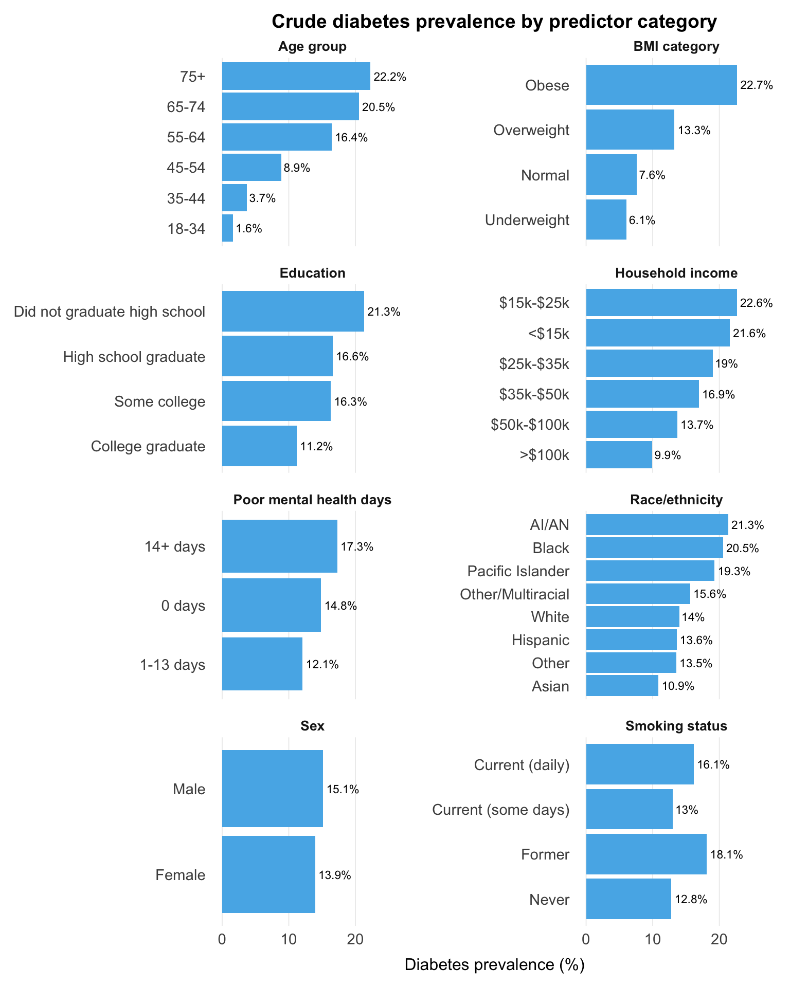
Prevalence climbs from 1.6% at ages 18-34 to 22.2% at 75+, and the BMI gradient is nearly as steep: 22.7% in the obese group versus 7.6% at normal weight. Prevalence also rises as income and education fall.
Behavioural and health indicators show further differences, including higher prevalence among former smokers and among those reporting 14+ poor mental health days, though these may reflect confounding or changes following diagnosis rather than independent effects. Variation across race and ethnicity is substantial but rests on small samples in several groups.
---
## Unadjusted Associations
Diabetes status is regressed on each predictor individually, producing a crude odds ratio (OR) for the association without adjustment for any other variable.
```{r}
#| label: uvregression
df |>
  mutate(
    diabetes          = factor(diabetes, levels = c(0, 1)),
    age_group         = factor(age_group,
                               levels = c("18-34", "35-44", "45-54", "55-64", "65-74", "75+")),
    sex               = factor(sex, levels = c("Male", "Female")),
    race_ethnicity    = factor(race_ethnicity, levels = c("White", "Black",
                                                          "American Indian/Alaskan Native",
                                                          "Asian", "Pacific Islander",
                                                          "Other/Multiracial",
                                                          "Hispanic", "Other")),
    education         = factor(education,
                               levels = c("College graduate", "Some college",
                                          "High school graduate", "Did not graduate high school")),
    income_group      = factor(income_group,
                               levels = c(">$100k", "$50k-$100k", "$35k-$50k",
                                          "$25k-$35k", "$15k-$25k", "<$15k")),
    bmi_category      = factor(bmi_category,
                               levels = c("Normal", "Underweight", "Overweight", "Obese")),
    smoking_status    = factor(smoking_status,
                               levels = c("Never", "Former", "Current (some days)", "Current (daily)")),
    mental_health_days = factor(mental_health_days,
                                levels = c("0 days", "1-13 days", "14+ days"))
  ) |>
  select(
    diabetes,
    age_group, sex, race_ethnicity, education, income_group,
    bmi_category, physically_active, smoking_status,
    heavy_drinker, has_provider, mental_health_days
  ) |>
  tbl_uvregression(
    method       = glm,
    y            = diabetes,
    method.args  = list(family = binomial),
    exponentiate = TRUE,
    estimate_fun = \(x) style_sigfig(x, digits = 3),
    label        = list(
      age_group          ~ "Age group",
      sex                ~ "Sex",
      race_ethnicity     ~ "Race/ethnicity",
      education          ~ "Education",
      income_group       ~ "Household income",
      bmi_category       ~ "BMI category",
      physically_active  ~ "Physically active",
      smoking_status     ~ "Smoking status",
      heavy_drinker      ~ "Heavy drinker",
      has_provider       ~ "Has personal doctor",
      mental_health_days ~ "Poor mental health days"
    )
  ) |>
  bold_p(t = 0.05) |>
  bold_labels() |>
  modify_caption("**Table 2.** Unadjusted odds ratios for diabetes by predictor")
```
The age odds ratio rises steadily from 2.29 in the 35-44 group to 17.2 in those aged 75+, and adults with obesity have 3.58 times the odds of those at normal weight. Odds also rise step by step as income and education fall.
As in the prevalence plots, the lower odds among physically active respondents and higher odds among former smokers likely reflect confounding and behaviour changes following diagnosis. Heavy drinking (OR 0.42) and having a personal doctor (OR 4.29) show clear signs of reverse causation: the direction of association fits disease status influencing behaviour or healthcare contact. These crude estimates provide context, but many will attenuate or change after adjustment.
---
## Missingness
The SQL pipeline recoded "don't know", "refused", and "not applicable" responses to `NULL`. Variables not shown have no missing values.
```{r}
#| label: missingness
miss_summary(df)
```
Income group stands out with 25.5% missingness, the only variable where nonresponse is large enough to meaningfully shrink the complete-case sample. Most other variables fall below 10%, with heavy drinking (10.2%) and BMI category (9.3%) adding some row loss. Whether income nonresponse is random or related to diabetes risk is unclear, but its scale matters when interpreting complete-case results.
---
## Summary
Age and BMI are the most consistent signals, with strong, monotonic gradients across the descriptive analyses. Socioeconomic predictors show clear unadjusted associations, while income group carries substantial missingness (25.5%) that shrinks the complete-case sample. Several behavioural variables, particularly heavy drinking and having a personal doctor, show patterns more consistent with reverse causation than independent effects.
The adjusted model will help separate these overlapping relationships and show which associations persist.
---
## Session Info
```{r}
#| label: session-info
#| collapse: true
#| code-summary: "R session info"
sessionInfo()
```