---
title: "{{< var study_title >}}"
subtitle: "Overview: Key Findings"
---
This analysis uses data from the 2024 Behavioral Risk Factor Surveillance System (BRFSS), a U.S. health survey of over 450,000 adults, to identify which demographic, socioeconomic, and behavioural factors are most strongly linked to a diabetes diagnosis after adjusting for the others. This page summarises the key findings; full methods and model diagnostics are in the [Logistic Regression notebook](logistic-regression.qmd).
```{r}
#| label: setup
#| include: false
library(here)
library(tidyverse)
library(broom)
library(pROC)
source(here("R", "utils.R"))
source(here("R", "plot_theme.R"))
mod <- readRDS(here("data", "processed", "mod.rds"))
df_cc <- readRDS(here("data", "processed", "df_cc.rds"))
roc_obj <- pROC::roc(
response = df_cc$diabetes == "Yes",
predictor = predict(mod, type = "response"),
quiet = TRUE
)
auc_val <- as.numeric(pROC::auc(roc_obj))
```
## Key Findings
**Age is the strongest predictor of diabetes risk.** Adults aged 75+ have `r round(exp(coef(mod)["age_group75+"]), 0)` times the odds of a diabetes diagnosis compared to those aged 18-34, after adjusting for other factors.
**Obesity and age compound risk.** Adults with an obese BMI have `r round(exp(coef(mod)["bmi_categoryObese"]), 1)` times the odds of a diagnosis compared to those at a normal weight, and this gap widens with age.
**Socioeconomic and racial disparities persist after adjustment.** Lower income is linked to higher risk, and several racial and ethnic groups show higher odds even after adjusting for income, education, and lifestyle.
**The model discriminates reliably but not perfectly.** It ranks a person with diabetes above a person without in `r round(auc_val * 100, 0)`% of cases.
---
## How diabetes risk changes across the population
The figures below show how diabetes risk changes with age, body weight, and income, and highlight a few key results from the full model.
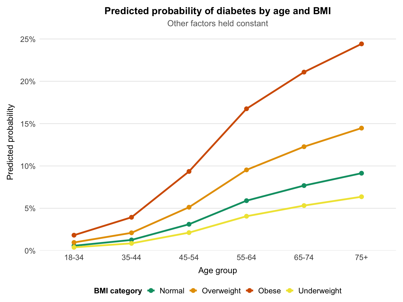
### Diabetes risk rises sharply with age and BMI
```{r}
#| label: viz-pred-prob
#| code-summary: "Build prediction grid and plot"
pred_grid <- expand.grid(
  age_group    = levels(df_cc$age_group),
  bmi_category = levels(df_cc$bmi_category)
) |>
  mutate(
    age_group          = factor(age_group,    levels = levels(df_cc$age_group)),
    bmi_category       = factor(bmi_category, levels = levels(df_cc$bmi_category)),
    sex                = factor("Male",             levels = levels(df_cc$sex)),
    race_ethnicity     = factor("White",            levels = levels(df_cc$race_ethnicity)),
    education          = factor("College graduate", levels = levels(df_cc$education)),
    income_group       = factor(">$100k",           levels = levels(df_cc$income_group)),
    physically_active  = factor("Active",           levels = levels(df_cc$physically_active)),
    smoking_status     = factor("Never",            levels = levels(df_cc$smoking_status)),
    heavy_drinker      = factor("No",               levels = levels(df_cc$heavy_drinker)),
    has_provider       = factor("Has provider",     levels = levels(df_cc$has_provider)),
    mental_health_days = factor("0 days",           levels = levels(df_cc$mental_health_days))
  )

pred_grid$prob <- predict(mod, newdata = pred_grid, type = "response")

ggplot(pred_grid, aes(x = age_group, y = prob,
                      color = bmi_category, group = bmi_category)) +
  geom_line(linewidth = 1.2) +
  geom_point(size = 2.5) +
  scale_y_continuous(
    labels = scales::percent_format(accuracy = 1),
    limits = c(0, NA),
    expand = expansion(mult = c(0, 0.05))
  ) +
  scale_color_manual(
    values = c(
      "Normal"      = palette_epi[["green"]],
      "Underweight" = palette_epi[["yellow"]],
      "Overweight"  = palette_epi[["orange"]],
      "Obese"       = palette_epi[["vermillion"]]
    ),
    breaks = c("Normal", "Overweight", "Obese", "Underweight"),
    name = "BMI category"
  ) +
  labs(
    title    = "Predicted probability of diabetes by age and BMI",
    subtitle = "Other factors held constant",
    x        = "Age group",
    y        = "Predicted probability"
  ) +
  theme_epi(grid = "y") +
  theme(
    plot.title    = element_text(hjust = 0.5),
    plot.subtitle = element_text(hjust = 0.5)
  )
```
Diabetes risk rises with both age and body weight, and the two effects build on each other. In this model, predicted risk for adults with obesity rises from `r round(pred_grid[pred_grid$age_group == "18-34" & pred_grid$bmi_category == "Obese", "prob"] * 100, 1)`% at age 18-34 to `r round(pred_grid[pred_grid$age_group == "75+" & pred_grid$bmi_category == "Obese", "prob"] * 100, 1)`% at age 75+, compared to `r round(pred_grid[pred_grid$age_group == "75+" & pred_grid$bmi_category == "Normal", "prob"] * 100, 1)`% for normal-weight adults of the same age.
These estimates hold other factors constant to isolate age and BMI. In practice, risk is higher for people with additional risk factors such as lower income, physical inactivity, or existing health conditions.
```{r}
#| label: or-data
#| include: false
or_df <- tidy(mod, exponentiate = TRUE) |>
filter(term != "(Intercept)") |>
mutate(
conf.low = estimate * exp(-1.96 * std.error),
conf.high = estimate * exp( 1.96 * std.error)
)
```
---
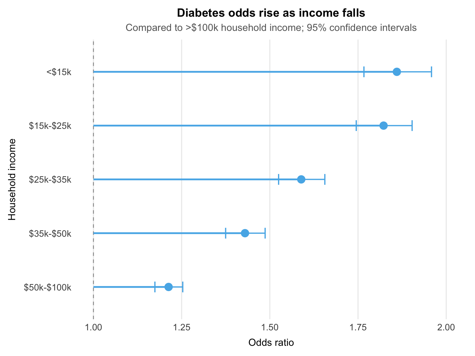
### Diabetes risk increases as income falls
```{r}
#| label: viz-income-gradient
#| code-summary: "Income gradient lollipop"
income_levels <- c("$50k-$100k", "$35k-$50k", "$25k-$35k", "$15k-$25k", "<$15k")

income_df <- or_df |>
  filter(str_detect(term, "^income_group")) |>
  mutate(
    label = factor(str_remove(term, "^income_group"), levels = income_levels)
  )

ggplot(income_df, aes(x = estimate, y = label)) +
  geom_vline(xintercept = 1, linetype = "dashed", color = "grey60", linewidth = 0.5) +
  geom_segment(aes(x = 1, xend = estimate, yend = label),
               color = palette_epi[["sky_blue"]], linewidth = 1) +
  geom_errorbarh(aes(xmin = conf.low, xmax = conf.high),
                 height = 0.2, color = palette_epi[["sky_blue"]], linewidth = 0.7) +
  geom_point(size = 4, color = palette_epi[["sky_blue"]]) +
  scale_x_continuous(expand = expansion(add = c(0.05, 0.1))) +
  labs(
    title    = "Diabetes odds rise as income falls",
    subtitle = "Compared to >$100k household income; 95% confidence intervals",
    x        = "Odds ratio",
    y        = "Household income"
  ) +
  theme_epi(grid = "x") +
  theme(
    plot.title    = element_text(hjust = 0.5),
    plot.subtitle = element_text(hjust = 0.5)
  )
```
Diabetes risk increases steadily as income falls, not just at the extremes. Adults with a household income below $15,000 have `r round(or_df$estimate[or_df$term == "income_group<$15k"], 2)` times the odds of a diabetes diagnosis compared to those earning over $100,000, and this gradient persists after adjusting for age, body weight, race, and lifestyle factors.
This suggests that income is not simply a proxy for individual behaviour, but is independently associated with diabetes risk.
---
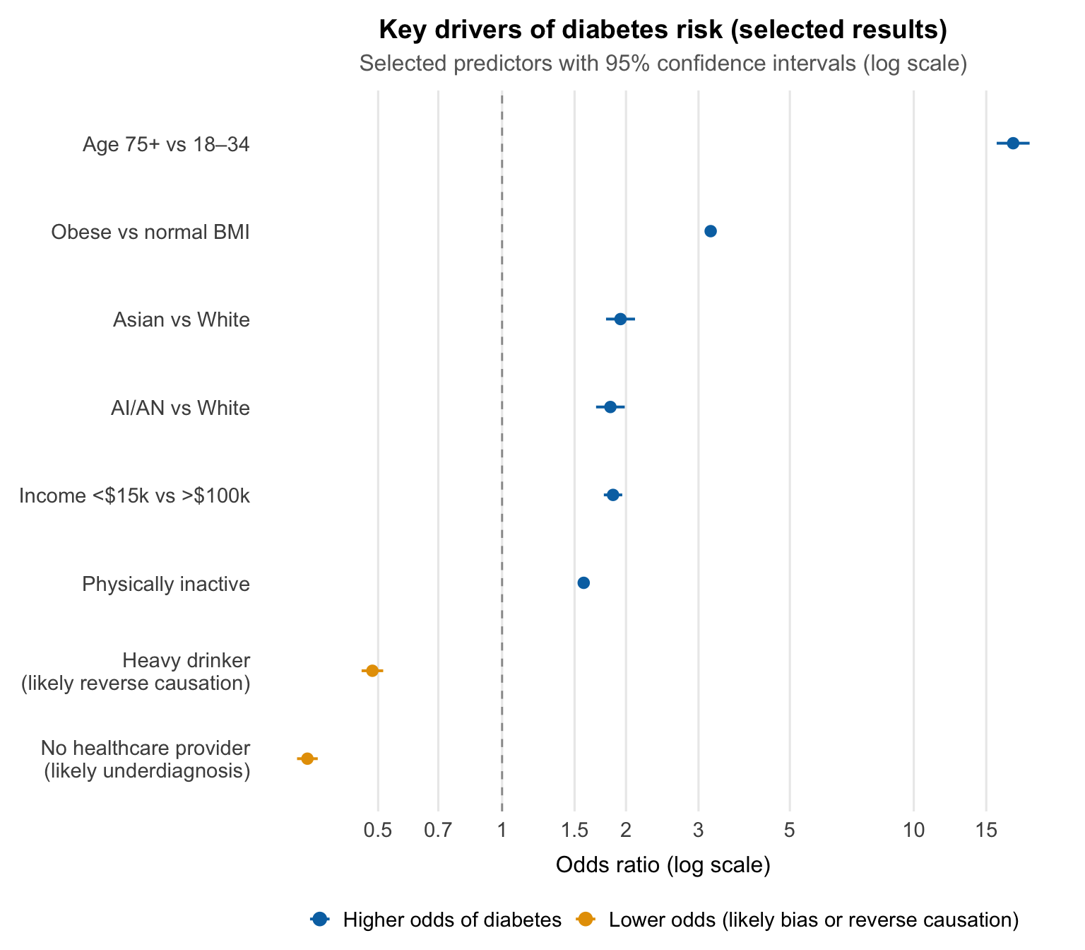
### Key drivers of diabetes risk
```{r}
#| label: viz-curated-forest
#| fig-height: 7
#| code-summary: "Curated forest plot"
curated_labels <- c(
  "age_group75+"                                 = "Age 75+ vs 18-34",
  "bmi_categoryObese"                            = "Obese vs normal BMI",
  "income_group<$15k"                            = "Income <$15k vs >$100k",
  "race_ethnicityAmerican Indian/Alaskan Native" = "AI/AN vs White",
  "race_ethnicityAsian"                          = "Asian vs White",
  "physically_activeInactive"                    = "Physically inactive",
  "has_providerNo provider"                      = "No healthcare provider\n(likely underdiagnosis)",
  "heavy_drinkerYes"                             = "Heavy drinker\n(likely reverse causation)"
)

curated_df <- or_df |>
  filter(term %in% names(curated_labels)) |>
  mutate(
    label = factor(curated_labels[term], levels = c(
      "No healthcare provider\n(likely underdiagnosis)",
      "Heavy drinker\n(likely reverse causation)",
      "Physically inactive",
      "Income <$15k vs >$100k",
      "AI/AN vs White",
      "Asian vs White",
      "Obese vs normal BMI",
      "Age 75+ vs 18-34"
    )),
    direction = if_else(estimate >= 1, "Higher odds of diabetes",
                                       "Lower odds (likely bias or reverse causation)")
  )

ggplot(curated_df, aes(x = estimate, y = label, color = direction)) +
  geom_vline(xintercept = 1, linetype = "dashed", color = "grey60", linewidth = 0.5) +
  geom_pointrange(aes(xmin = conf.low, xmax = conf.high), linewidth = 0.7, fatten = 3) +
  scale_x_log10(
    breaks = c(0.5, 0.7, 1, 1.5, 2, 3, 5, 10, 15),
    labels = c("0.5", "0.7", "1", "1.5", "2", "3", "5", "10", "15")
  ) +
  scale_color_manual(
    values = c(
      "Higher odds of diabetes"                    = palette_epi[["blue"]],
      "Lower odds (likely bias or reverse causation)" = palette_epi[["orange"]]
    ),
    name = NULL
  ) +
  labs(
    title    = "Key drivers of diabetes risk (selected results)",
    subtitle = "Selected predictors with 95% confidence intervals (log scale)",
    x        = "Odds ratio (log scale)",
    y        = NULL
  ) +
  theme_epi(grid = "x") +
  theme(
    plot.title    = element_text(hjust = 0.5),
    plot.subtitle = element_text(hjust = 0.5)
  )
```
Age is the strongest predictor in the model: adults aged 75 and over have `r round(exp(coef(mod)["age_group75+"]), 0)` times the odds of a diabetes diagnosis compared to those aged 18-34. Obesity, income, racial and ethnic background, and physical inactivity are also independently associated with higher risk.
Two findings show lower odds, but neither is protective. People without a regular healthcare provider are less likely to be diagnosed whatever their underlying risk, which points to underdiagnosis. The heavy-drinking result likely reflects reverse causation: people with chronic illness often cut back on alcohol, so current heavy drinkers look healthier on average than they are.
These results show that diabetes risk is shaped by age, body weight, and socioeconomic conditions together. Some associations reflect underlying biology; others show how access to care and behaviour shape what appears in the data.