---
title: "Modelling Diabetes Risk: Social and Behavioural Factors in BRFSS Data"
subtitle: "Multivariable Logistic Regression Analysis · n = 287,804"
---
This notebook estimates adjusted associations between diabetes status and demographic, socioeconomic, and behavioural predictors using multivariable logistic regression.
The data come from the 2024 Behavioral Risk Factor Surveillance System (BRFSS), a nationally representative telephone survey of U.S. adults conducted annually by the CDC. The analysis examines whether these factors remain associated with diabetes status after adjustment for confounding.
## Setup
```{r}
#| label: setup
#| collapse: true
#| code-summary: "Load packages and helpers"
library(here)
library(tidyverse)
library(arrow)
library(gtsummary)
library(janitor)
library(broom)            # tidy(): extract model coefficients as a data frame
library(car)              # vif(): variance inflation factors
library(performance)      # check_model(): visual diagnostic plots
library(see)              # plotting backend for performance
library(patchwork)        # plot composition and annotation
library(pROC)             # roc(), auc(), ggroc(): ROC curve and AUC
library(ResourceSelection) # hoslem.test(): Hosmer-Lemeshow goodness-of-fit

source(here("R", "utils.R"))
source(here("R", "plot_theme.R"))
```
`car` checks multicollinearity via variance inflation factors, and `performance` provides diagnostic plots to assess overall model behaviour. `pROC` evaluates discrimination through the ROC curve and AUC, and `ResourceSelection` provides the Hosmer-Lemeshow test as a basic check of calibration across risk strata.
Model estimates are extracted with `broom` and presented using `gtsummary` for consistent reporting.
---
## Data Import
```{r}
#| label: import
#| collapse: true
df_raw <- read_parquet(here("data", "processed", "analysis_dataset.parquet"))
cat("Rows:", nrow(df_raw), "| Columns:", ncol(df_raw), "\n")
```
The analytical dataset is produced by the SQL pipeline from the raw 2024 BRFSS XPT file. Respondents with a missing or ambiguous diabetes response are excluded at the SQL stage, so all `r format(nrow(df_raw), big.mark = ",")` rows carry a definitive binary outcome. No further row-level exclusions are applied until the complete-case step in Data Preparation.
---
## Data Preparation
### Factor levels and reference categories
Reference categories determine the comparison group for each odds ratio. We set these to meaningful baselines (typically the lowest-risk or most advantaged group) so that estimated effects read as higher risk relative to a favourable exposure level, keeping the direction of associations intuitive.
```{r}
#| label: prep-factors
#| code-summary: "Set factor levels and reference categories"
df <- df_raw |>
  mutate(
    diabetes = factor(diabetes, levels = c(0, 1), labels = c("No", "Yes")),

    age_group = factor(age_group,
                       levels = c("18-34", "35-44", "45-54", "55-64", "65-74", "75+")),

    sex = factor(sex, levels = c("Male", "Female")),

    race_ethnicity = factor(race_ethnicity,
                            levels = c("White", "Black",
                                       "American Indian/Alaskan Native",
                                       "Asian", "Pacific Islander",
                                       "Other/Multiracial",
                                       "Hispanic", "Other")),

    education = factor(education,
                       levels = c("College graduate", "Some college",
                                  "High school graduate", "Did not graduate high school")),

    income_group = factor(income_group,
                          levels = c(">$100k", "$50k-$100k", "$35k-$50k",
                                     "$25k-$35k", "$15k-$25k", "<$15k")),

    bmi_category = factor(bmi_category,
                          levels = c("Normal", "Underweight", "Overweight", "Obese")),

    physically_active = factor(physically_active, levels = c(1, 0),
                               labels = c("Active", "Inactive")),

    smoking_status = factor(smoking_status,
                            levels = c("Never", "Former",
                                       "Current (some days)", "Current (daily)")),

    heavy_drinker = factor(heavy_drinker, levels = c(0, 1),
                           labels = c("No", "Yes")),

    has_provider = factor(has_provider, levels = c(1, 0),
                          labels = c("Has provider", "No provider")),

    mental_health_days = factor(mental_health_days,
                                levels = c("0 days", "1-13 days", "14+ days"))
  )
```
The first level of each factor becomes the reference category under R’s default treatment coding. This choice affects how contrasts are expressed, but does not change overall model fit.
### Complete-case exclusions
`glm()` cannot use rows with missing values, so any row missing a predictor is dropped here. The retained dataset `df_cc` is used for all subsequent modelling.
```{r}
#| label: complete-cases
#| collapse: true
predictor_cols <- c(
"age_group", "sex", "race_ethnicity", "education", "income_group",
"bmi_category", "physically_active", "smoking_status",
"heavy_drinker", "has_provider", "mental_health_days"
)
n_before <- nrow(df)
df_cc <- df |> drop_na(all_of(predictor_cols))
n_after <- nrow(df_cc)
cat("Before:", n_before, "| After:", n_after, "| Excluded:", n_before - n_after,
"(", round((n_before - n_after) / n_before * 100, 1), "%)\n")
```
`r round((nrow(df) - nrow(df_cc)) / nrow(df) * 100, 1)`% of respondents are excluded, largely due to the 25.5% income-group missingness identified in the EDA. The reason for this missingness is unknown; if lower-income respondents are more likely to skip the question, the estimated income gradient may be attenuated, and the reverse would inflate it. This is the main limitation of the complete-case approach.
---
## Model Specification
The outcome, diabetes diagnosis, is binary, so logistic regression models the log-odds of diagnosis as a function of the predictors. Coefficients are exponentiated and reported as odds ratios (ORs), the standard effect measure for this kind of cross-sectional analysis.
All 11 predictors are entered simultaneously rather than selected stepwise. Stepwise procedures can improve apparent fit in-sample but tend to produce unstable estimates and inflated Type I error. The aim here is to estimate the adjusted association of each predictor with diabetes status, so a theory-driven full model is preferred.
The model includes three demographic predictors (age, sex, race/ethnicity), two socioeconomic predictors (education and income), one access-to-care predictor (having a personal doctor), and five behavioural and clinical predictors (BMI, physical activity, smoking, alcohol use, and mental health).
```{r}
#| label: model-formula
model_formula <- formula(
  diabetes ~
    age_group + sex + race_ethnicity +
    education + income_group + has_provider +
    bmi_category + physically_active + smoking_status +
    heavy_drinker + mental_health_days
)
model_formula
```
This is an associational model fit to cross-sectional data: it estimates adjusted odds, not causal effects. Diabetes status and the predictors are measured at the same point in time, so the direction of causality cannot be established from these data alone.
---
## Model Fitting
The specified logistic regression model is fit to the complete-case dataset.
```{r}
#| label: model-fit
#| collapse: true
mod <- glm(model_formula, data = df_cc, family = binomial(link = "logit"))
saveRDS(mod, here("data", "processed", "mod.rds"))
saveRDS(df_cc, here("data", "processed", "df_cc.rds"))
cat("Converged:", mod$converged, "\n")
glance(mod)
```
The model converged successfully. The reduction in deviance relative to the null model indicates that the predictors collectively improve model fit. Adjusted associations are interpreted in the Results section, after diagnostic checks.
---
## Assumption Checks
Model fit alone does not guarantee reliable estimates, so key assumptions are checked before interpreting coefficients.
### Multicollinearity: VIF
Highly correlated predictors inflate standard errors and make individual coefficients unstable, even when overall model fit is acceptable. Variance inflation factors (VIFs) quantify this inflation for each predictor.
```{r}
#| label: assumption-vif
#| collapse: true
vif(mod)
```
Because several predictors are multi-level categorical variables, `car::vif()` reports generalised VIFs (GVIF). The adjusted values, GVIF^(1/(2·Df)), are all below 1.05, well under the conventional threshold of 2, indicating no meaningful collinearity.
Income and education show slightly higher values than the other predictors, consistent with their expected correlation in the population, but neither approaches a level that would inflate standard errors or destabilise coefficient estimates.
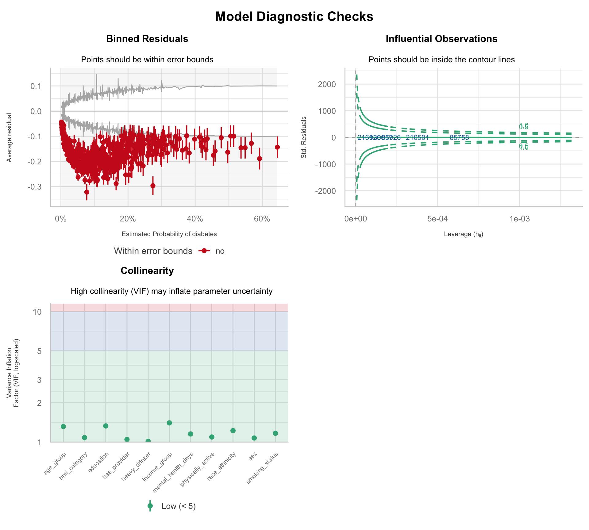
### Model diagnostics
Three diagnostic panels assess model fit, influential observations, and collinearity before interpreting coefficients.
```{r}
#| label: assumption-diagnostics
#| fig-width: 10
#| fig-height: 9
#| fig-keep: last
cm <- check_model(mod, check = c("binned_residuals", "outliers", "vif"),
                  residual_type = "normal")

diag_plot <- plot(cm) &
  theme(
    plot.title    = element_text(size = 12, face = "bold", hjust = 0.5),
    plot.subtitle = element_text(size = 10, hjust = 0.5),
    axis.title    = element_text(size = 8),
    plot.margin   = margin(t = 8, r = 8, b = 8, l = 8)
  )

diag_plot[[3]] <- diag_plot[[3]] +
  theme(
    plot.subtitle = element_text(size = 10, hjust = 0.5, margin = margin(b = 10, l = 60)),
    axis.text.x   = element_text(angle = 45, hjust = 1, vjust = 1, size = 7.5),
    plot.margin   = margin(t = 8, r = 8, b = 18, l = 8)
  )

diag_plot +
  patchwork::plot_annotation(
    title = "Model Diagnostic Checks",
    theme = theme(
      plot.title  = element_text(size = 16, face = "bold", hjust = 0.5),
      plot.margin = margin(t = 14, b = 8)
    )
  )
```
The binned residuals plot shows systematic deviation outside the error bounds, with residuals consistently negative across the predicted probability range. The model overpredicts diabetes probability across most of the risk distribution: the linear functional form does not fully capture the relationship between the predictors and the log-odds of the outcome.
This pattern is consistent with non-linear associations in key predictors (particularly age, BMI, and mental health days) and the absence of interaction terms in the current specification. No influential observations are identified in the Cook's distance panel, as expected given the sample size.
This misfit does not invalidate the model, but it suggests that effect estimates should be interpreted with caution.
---
## Results
### Adjusted odds ratios
The primary result of this analysis is the set of adjusted ORs from the full multivariable model: the estimated odds of diabetes for each predictor level, holding all other predictors constant.
```{r}
#| label: results-adjusted
tbl_regression(
  mod,
  exponentiate = TRUE,
  estimate_fun = \(x) style_sigfig(x, digits = 3),
  label = list(
    age_group          ~ "Age group",
    sex                ~ "Sex",
    race_ethnicity     ~ "Race/ethnicity",
    education          ~ "Education",
    income_group       ~ "Household income",
    bmi_category       ~ "BMI category",
    physically_active  ~ "Physically active",
    smoking_status     ~ "Smoking status",
    heavy_drinker      ~ "Heavy drinker",
    has_provider       ~ "Has personal doctor",
    mental_health_days ~ "Poor mental health days"
  )
) |>
  bold_p(t = 0.05) |>
  bold_labels() |>
  modify_caption("**Table 1.** Adjusted odds ratios from the full social determinants model")
```
The adjusted model shows the strongest associations for BMI and age, with obesity and older age groups carrying substantially higher odds of diabetes than their reference categories. Lower income groups also retain elevated odds after adjustment, indicating that the socioeconomic gradient is not fully explained by the behavioural and clinical predictors in the model. Several smaller effects remain directionally consistent with the EDA, though their magnitude and precision vary once the predictors are considered jointly.
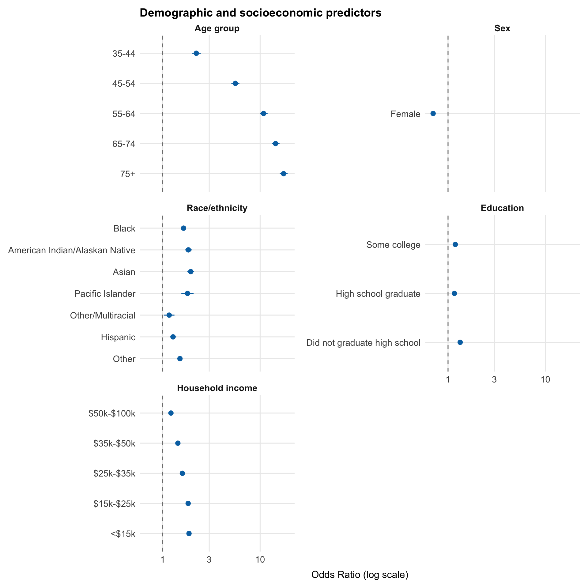
### Forest plot
A visual complement to Table 1. Points show adjusted odds ratios for each predictor level, with horizontal bars representing 95% confidence intervals. The dashed line at OR = 1 marks the null (no association), and the x-axis is on a log scale, so equal distances represent equal multiplicative changes in odds. Predictors are split across two figures by domain.
```{r}
#| label: results-forest-demo
#| fig-cap: "Adjusted ORs with 95% CIs: demographic and socioeconomic predictors"
#| fig-width: 10
#| fig-height: 10
predictor_names <- c(
  "age_group", "sex", "race_ethnicity", "education", "income_group",
  "bmi_category", "physically_active", "smoking_status",
  "heavy_drinker", "mental_health_days", "has_provider"
)

var_labels <- c(
  age_group          = "Age group",
  sex                = "Sex",
  race_ethnicity     = "Race/ethnicity",
  education          = "Education",
  income_group       = "Household income",
  bmi_category       = "BMI category",
  physically_active  = "Physically active",
  smoking_status     = "Smoking status",
  heavy_drinker      = "Heavy drinker",
  mental_health_days = "Poor mental health days",
  has_provider       = "Has personal doctor"
)

demo_vars <- c("age_group", "sex", "race_ethnicity", "education", "income_group")

forest_data <- tidy(mod, conf.int = TRUE, exponentiate = TRUE) |>
  filter(term != "(Intercept)") |>
  mutate(
    variable = str_extract(term, str_c("^(", str_c(predictor_names, collapse = "|"), ")")),
    label    = str_remove(term, variable),
    variable = factor(variable, levels = predictor_names)
  ) |>
  arrange(variable)

forest_demo <- filter(forest_data, variable %in% demo_vars)

ggplot(forest_demo,
       aes(x = estimate,
           y = fct_rev(factor(term, levels = unique(term))),
           xmin = conf.low, xmax = conf.high)) +
  geom_vline(xintercept = 1, linetype = "dashed", color = "grey50") +
  geom_pointrange(color = palette_epi[["blue"]], size = 0.4) +
  facet_wrap(~variable, scales = "free_y", ncol = 2,
             labeller = as_labeller(var_labels)) +
  scale_x_log10() +
  scale_y_discrete(labels = \(x) forest_data$label[match(x, forest_data$term)]) +
  labs(x = "Odds Ratio (log scale)", y = NULL,
       title = "Demographic and socioeconomic predictors")
```
The demographic and socioeconomic panel shows a clear gradient in diabetes risk. Age is the dominant predictor, with odds increasing sharply and monotonically across older age groups. Income and education show consistent inverse gradients, with lower socioeconomic status associated with higher odds of diabetes.
Race and ethnicity show elevated adjusted odds across most groups, with Asian, AI/AN, Black, and Pacific Islander respondents all above OR 1.6 relative to White respondents. Intervals are wider for smaller subgroups, consistent with the uneven sample composition seen in the EDA. Sex shows a precisely estimated association in the expected direction: female respondents have roughly 30% lower adjusted odds, smaller than the age or BMI effects but not negligible.
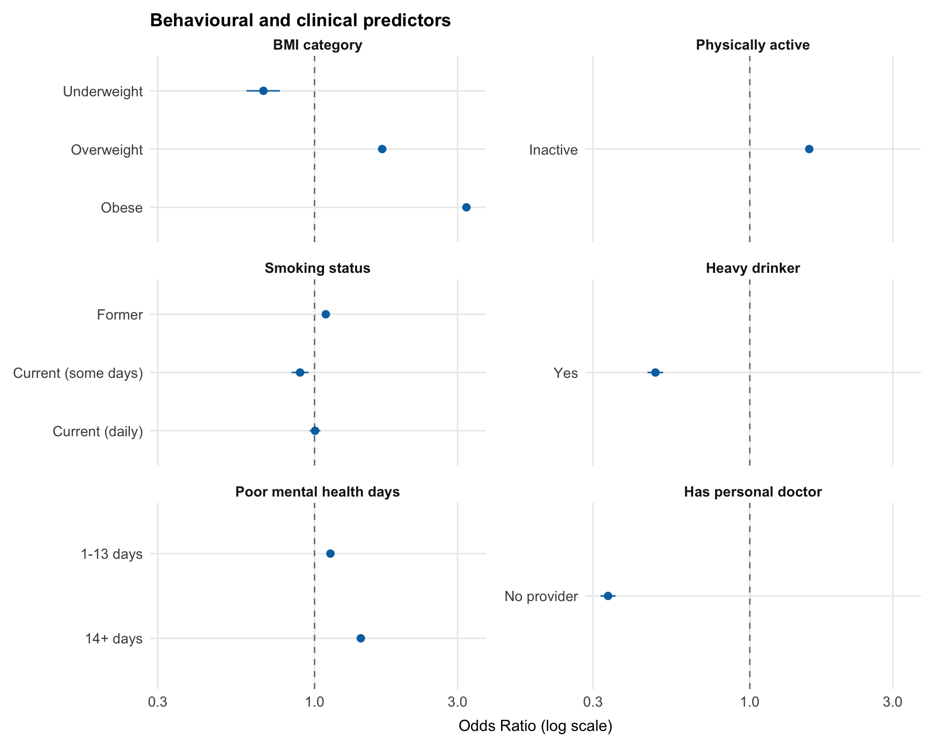
```{r}
#| label: results-forest-behav
#| fig-cap: "Adjusted ORs with 95% CIs: behavioural and clinical predictors"
#| fig-width: 10
#| fig-height: 8
behav_vars <- c("bmi_category", "physically_active", "smoking_status",
                "heavy_drinker", "mental_health_days", "has_provider")

forest_behav <- filter(forest_data, variable %in% behav_vars)

ggplot(forest_behav,
       aes(x = estimate,
           y = fct_rev(factor(term, levels = unique(term))),
           xmin = conf.low, xmax = conf.high)) +
  geom_vline(xintercept = 1, linetype = "dashed", color = "grey50") +
  geom_pointrange(color = palette_epi[["blue"]], size = 0.4) +
  facet_wrap(~variable, scales = "free_y", ncol = 2,
             labeller = as_labeller(var_labels)) +
  scale_x_log10() +
  scale_y_discrete(labels = \(x) forest_data$label[match(x, forest_data$term)]) +
  labs(x = "Odds Ratio (log scale)", y = NULL,
       title = "Behavioural and clinical predictors")
```
The behavioural and clinical panel is dominated by BMI, which shows a strong gradient in risk. Odds of diabetes increase substantially from overweight to obese, while underweight is associated with lower odds, making BMI the largest modifiable predictor in the model.
Physical inactivity and poor mental health are both associated with higher odds of diabetes, with mental health showing a graded pattern across categories. These effects are smaller than BMI but remain consistent in direction.
Smoking shows a non-monotonic pattern, with former smokers at higher odds than current smokers. This is consistent with reverse causation: people may quit smoking after diagnosis. Similar patterns appear for heavy drinking and having a personal doctor; neither is plausibly causal, and both are better explained by behaviour change or healthcare access following diagnosis.
### Unadjusted vs adjusted comparison
Comparing unadjusted and adjusted odds ratios highlights confounding: where an estimate changes after adjustment, part of the crude association was explained by other variables in the model.
```{r}
#| label: results-comparison
tbl_uv <- df_cc |>
  select(diabetes, all_of(predictor_cols)) |>
  tbl_uvregression(
    method       = glm,
    y            = diabetes,
    method.args  = list(family = binomial),
    exponentiate = TRUE,
    estimate_fun = \(x) style_sigfig(x, digits = 3),
    label = list(
      age_group          ~ "Age group",
      sex                ~ "Sex",
      race_ethnicity     ~ "Race/ethnicity",
      education          ~ "Education",
      income_group       ~ "Household income",
      bmi_category       ~ "BMI category",
      physically_active  ~ "Physically active",
      smoking_status     ~ "Smoking status",
      heavy_drinker      ~ "Heavy drinker",
      has_provider       ~ "Has personal doctor",
      mental_health_days ~ "Poor mental health days"
    )
  ) |>
  bold_p(t = 0.05)

tbl_mv <- tbl_regression(
  mod,
  exponentiate = TRUE,
  estimate_fun = \(x) style_sigfig(x, digits = 3),
  label = list(
    age_group          ~ "Age group",
    sex                ~ "Sex",
    race_ethnicity     ~ "Race/ethnicity",
    education          ~ "Education",
    income_group       ~ "Household income",
    bmi_category       ~ "BMI category",
    physically_active  ~ "Physically active",
    smoking_status     ~ "Smoking status",
    heavy_drinker      ~ "Heavy drinker",
    has_provider       ~ "Has personal doctor",
    mental_health_days ~ "Poor mental health days"
  )
) |>
  bold_p(t = 0.05)

tbl_merge(
  list(tbl_uv, tbl_mv),
  tab_spanner = c("**Unadjusted OR**", "**Adjusted OR**")
) |>
  bold_labels() |>
  modify_caption("**Table 2.** Unadjusted and adjusted odds ratios")
```
Several socioeconomic and behavioural effects attenuate after adjustment, particularly income, education, physical activity, and smoking, indicating that part of their crude association was shared with age and BMI.
In contrast, age and BMI remain strong with only modest attenuation, suggesting these are more robust associations in the data. The age gradient persists after adjustment, with the 75+ group retaining an OR of 17.4. The obesity effect is similarly stable (3.52 → 3.21), remaining the largest modifiable predictor in the model.
Some predictors change direction or strengthen after adjustment, highlighting more complex confounding. Asian ethnicity shifts from a protective crude association to elevated adjusted odds (0.79 → 1.94). This reflects confounding by socioeconomic status: in the crude analysis, higher average income and education levels suppress the underlying association, which becomes visible after adjustment. The 1-13 mental health day group shows a weaker reversal (0.76 → 1.13), likely reflecting adjustment for correlated behavioural and social factors. Reversals like these are why the crude-to-adjusted comparison is more than a formality in observational analyses.
---
## Model Performance
Model performance is assessed in terms of discrimination and calibration before interpreting predicted probabilities.
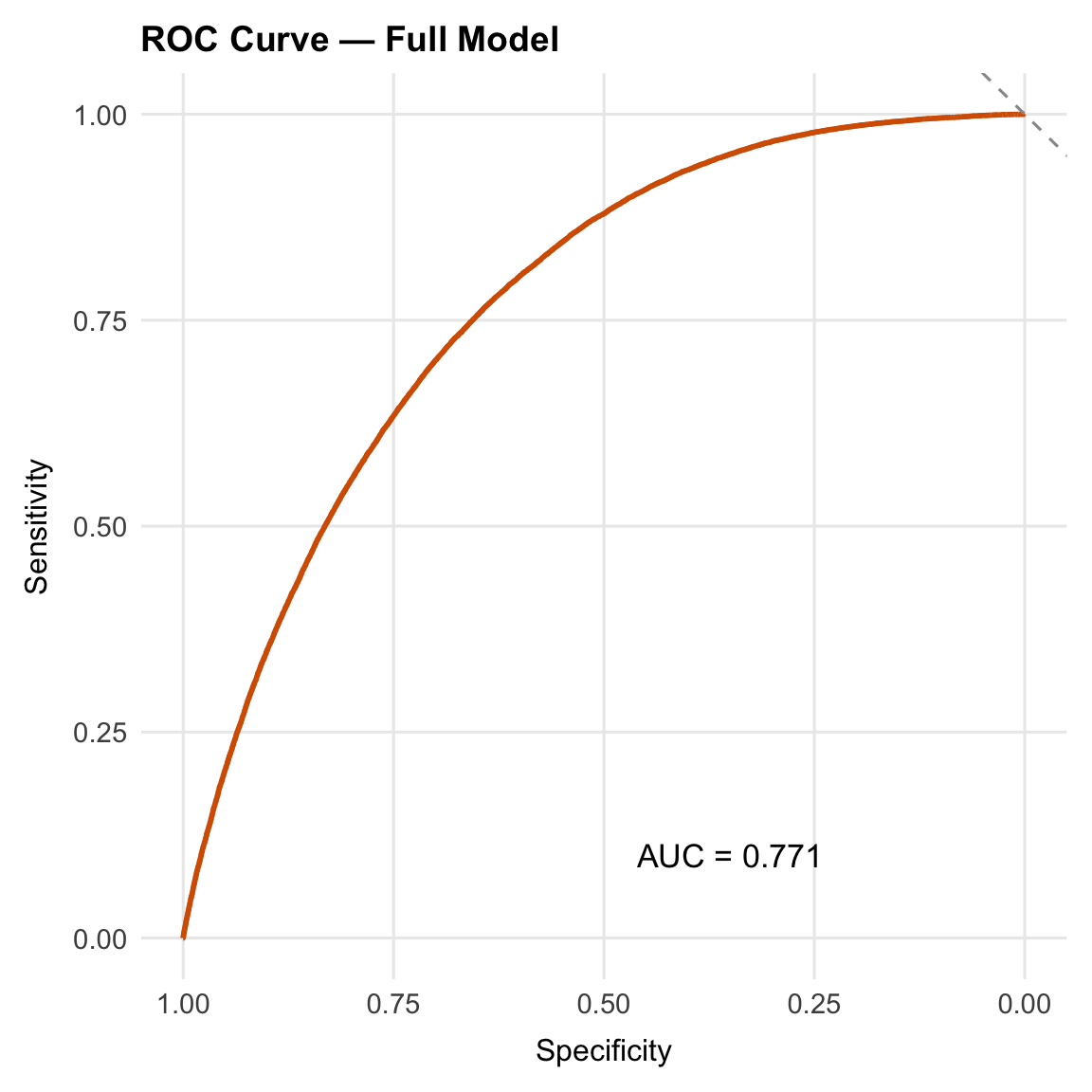
### Discrimination: ROC curve and AUC
The ROC curve and AUC assess whether the model assigns higher predicted probabilities to respondents with diabetes, indicating how well it ranks risk across the sample.
```{r}
#| label: performance-roc
#| fig-cap: "ROC curve: full social determinants model"
#| fig-width: 6
#| fig-height: 6
roc_obj <- roc(
  response  = as.integer(df_cc$diabetes) - 1L,
  predictor = fitted(mod),
  quiet     = TRUE
)

ggroc(roc_obj, color = palette_epi[["vermillion"]], linewidth = 1) +
  geom_abline(slope = -1, intercept = 1, linetype = "dashed", color = "grey60") +
  annotate("text", x = 0.35, y = 0.1,
           label = paste0("AUC = ", round(auc(roc_obj), 3)),
           size = 4.5) +
  labs(title = "ROC Curve: Full Model", x = "Specificity", y = "Sensitivity")
```
The model achieves an AUC of 0.771: if a respondent with diabetes and a respondent without are selected at random, the model assigns a higher predicted probability to the case 77.1% of the time. The predictors are demographic, socioeconomic, and self-reported behavioural measures, none of which directly measure metabolic function; clinical markers such as fasting glucose or HbA1c are not available in BRFSS. The next section quantifies how much the socioeconomic and behavioural predictors contribute beyond age, sex, and race/ethnicity alone.
### Incremental value of the social and behavioural predictors
A base model including age, sex, and race/ethnicity provides a reference point. Comparing its AUC with the full model's shows how much discrimination the socioeconomic and behavioural predictors add.
```{r}
#| label: performance-auc-comparison
#| collapse: true
mod_base <- glm(
diabetes ~ age_group + sex + race_ethnicity,
data = df_cc,
family = binomial
)
roc_base <- roc(
response = as.integer(df_cc$diabetes) - 1L,
predictor = fitted(mod_base),
quiet = TRUE
)
cat("Base model AUC (age + sex + race/ethnicity):", round(auc(roc_base), 3), "\n")
cat("Full model AUC (all predictors): ", round(auc(roc_obj), 3), "\n")
cat("Delta AUC: ", round(auc(roc_obj) - auc(roc_base), 3), "\n\n")
roc.test(roc_obj, roc_base)
```
The base model (age, sex, race/ethnicity) achieves an AUC of 0.696, compared with 0.771 for the full model (ΔAUC = 0.075).
The DeLong test confirms that this difference is not due to sampling variation (p < 0.001), but the magnitude is more informative than the p-value here: the added predictors improve risk ranking, but do not fundamentally change the model’s ability to separate cases from non-cases.
### Calibration
The Hosmer-Lemeshow test compares observed and expected event counts across deciles of predicted risk. A significant p-value indicates a difference between predicted and observed rates within these groups.
At this sample size (`r format(nrow(df_cc), big.mark = ",")`), the test has sufficient power to detect very small deviations, so a near-zero p-value is expected even when calibration is visually close. The p-value alone is insufficient; the calibration plot provides the more complete picture.
```{r}
#| label: performance-calibration
#| fig-cap: "Calibration plot: mean predicted probability vs observed proportion by decile"
#| fig-width: 6
#| fig-height: 6
cal_data <- tibble(
  predicted = fitted(mod),
  observed  = as.integer(df_cc$diabetes) - 1L
) |>
  mutate(decile = ntile(predicted, 10)) |>
  summarise(
    mean_pred = mean(predicted),
    mean_obs  = mean(observed),
    n         = n(),
    .by       = decile
  )

ggplot(cal_data, aes(x = mean_pred, y = mean_obs)) +
  geom_abline(slope = 1, intercept = 0, linetype = "dashed", color = "grey50") +
  geom_point(aes(size = n), color = palette_epi[["blue"]], show.legend = FALSE) +
  geom_line(color = palette_epi[["blue"]], linewidth = 0.5) +
  scale_x_continuous(labels = scales::percent_format()) +
  scale_y_continuous(labels = scales::percent_format()) +
  labs(x = "Mean predicted probability", y = "Observed proportion",
       title = "Calibration plot: predicted vs observed\n(by decile of predicted risk)") +
  theme(plot.title = element_text(hjust = 0.5))
```
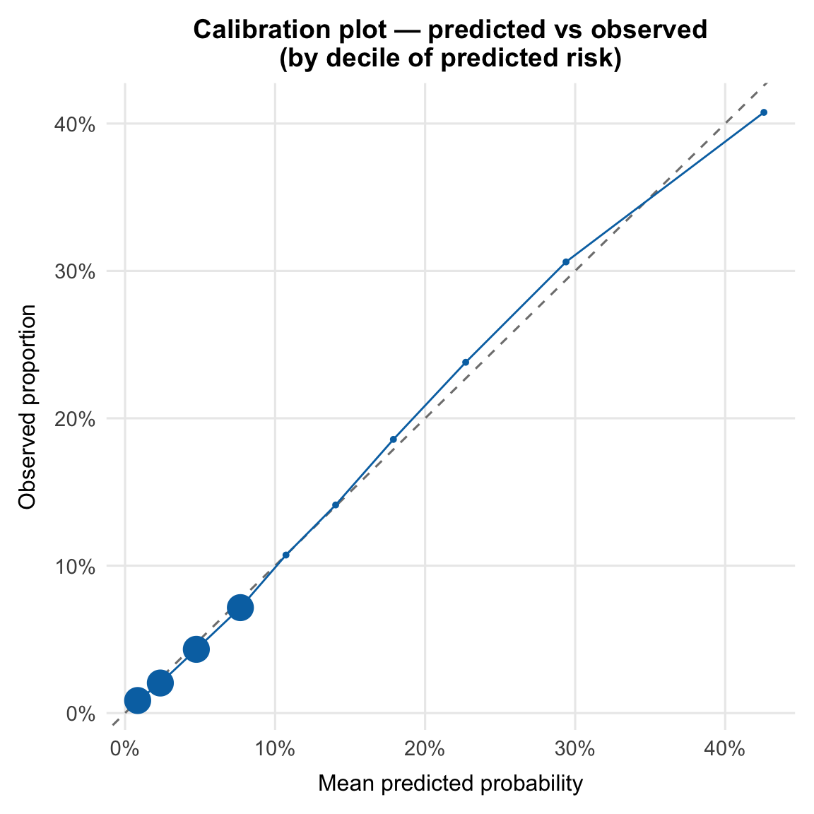
The calibration plot compares predicted probabilities with observed event rates across deciles of risk. Points close to the 45° line indicate good agreement; systematic deviation above the line indicates underprediction, and below indicates overprediction. Point size reflects the number of respondents in each decile.
Predicted probabilities are slightly elevated in the lower-risk deciles and modestly underestimated at the upper end, but remain close to the reference line across the full range. These deviations are small, and the model is well calibrated for population-level interpretation.
```{r}
#| label: performance-hosmer-lemeshow
#| collapse: true
hl <- hoslem.test(as.integer(df_cc$diabetes) - 1L, fitted(mod), g = 10)
print(hl)
```
The test returns X² = 124.21 (df = 8, p < 0.001). As expected at this sample size, the result is significant and reflects small deviations from perfect calibration.
Taken together, these checks address two questions: whether the model separates higher- from lower-risk respondents, and whether predicted probabilities align with observed rates. Here, they matter less for classification and more as evidence that the model is behaving consistently enough to support interpretation of the adjusted odds ratios.
---
## Conclusions
### Key findings
Obesity carries the highest adjusted odds in the model, with respondents in the obese BMI category having 3.21 times the odds of a diabetes diagnosis compared to those at normal weight. Age shows the steepest gradient: adjusted odds rise through each successive band, reaching OR 17.4 for the 75+ group relative to 18-34 year olds.
A clear income gradient persists after adjustment, with odds increasing from OR 1.21 in the $50k-$100k group to OR 1.86 in the lowest income bracket, compared to respondents earning over $100k. Racial and ethnic disparities are similarly robust, with Asian, American Indian or Alaska Native, and Black respondents all showing elevated adjusted odds relative to White respondents (OR 1.94, 1.83, and 1.63, respectively), so these associations are not fully explained by the socioeconomic and behavioural variables in the model.
Physical inactivity and poor mental health are independently associated with higher odds (OR 1.58 and 1.43 for 14+ poor mental health days, respectively). In contrast, two predictors show inverse associations: having no personal doctor (OR 0.337) and heavy drinking (OR 0.484). These are unlikely to reflect protective effects. Respondents without a provider are less likely to have received a diagnosis, while the heavy drinking association likely reflects detection bias or behavioural change following diagnosis. Former smokers show modestly elevated odds (OR 1.09), consistent with a similar pattern of cessation after diagnosis.
### Model performance
The full model achieves an AUC of `r round(auc(roc_obj), 3)`, compared to `r round(auc(roc_base), 3)` for the base demographic model, confirming that socioeconomic and behavioural predictors add meaningful discrimination beyond age, sex, and race/ethnicity alone. The calibration plot shows predicted probabilities are well aligned with observed rates across the risk distribution. The Hosmer-Lemeshow p-value is significant, as expected at this sample size, and does not indicate poor fit.
### Limitations
**Cross-sectional design.** Diabetes status and all predictors are measured at the same point in time. The direction of causality cannot be established. For example, diabetes diagnosis may prompt changes in physical activity or diet rather than the reverse.
**Unweighted analysis.** BRFSS uses a complex survey design with stratification, clustering, and post-stratification weights to produce nationally representative estimates. This analysis uses unweighted logistic regression, which produces valid associations within the sample but does not account for the survey design. Population-level prevalence estimates and fully representative ORs would require `svyglm()` from the `survey` package with the provided `psu`, `strata`, and `llcp_weight` variables.
**Self-reported outcome.** Diabetes status is based on self-report of a prior diagnosis. Undiagnosed diabetes, estimated to affect roughly 1 in 4 people with the condition, is not captured, which likely biases associations involving healthcare access towards the null.
**Complete-case analysis.** Respondents with missing predictor values were excluded (36.5%, n = 165,437), driven primarily by income-group nonresponse. If lower-income respondents are more likely to skip the question, the income gradient may be attenuated; the opposite pattern would inflate it. The missingness mechanism cannot be verified from these data.
---
## Session Info
```{r}
#| label: session-info
#| collapse: true
#| code-summary: "R session info"
sessionInfo()
```