---
title: "Exploratory Data Analysis"
subtitle: "{{< var study_title >}}"
---
## Setup
The following packages are loaded for this analysis. `arrow` enables reading from the parquet format used for the processed data mart. `gtsummary` produces publication-ready summary tables. `GGally` extends ggplot2 with the `ggpairs()` function used for the correlation matrix. A custom plot theme and colour palette are sourced from `R/plot_theme.R`.
```{r}
#| label: setup
#| collapse: true
#| code-summary: "Load packages and helpers"
library(here) # gives relative file paths from project root
library(tidyverse) # data manipulation and visualisation
library(arrow) # reads parquet files
library(skimr) # skim() for descriptive stats and missingness
library(janitor) # for tabulations
library(gtsummary) # for Table 1
library(GGally) # for correlation matrix

source(here("R", "plot_theme.R")) # palette_epi, theme_epi(), scale_*_epi()
```
---
## Data Import
Raw NHANES parquet files were downloaded using `R/download_raw.R`. The mart was built using DuckDB with four SQL scripts run in sequence: views over the raw parquet files, a join and recode to produce the analytical dataset, validation checks, and export to parquet for use in R.
```{sql}
--| label: sql-load-raw
--| code-summary: "01 - Create views over raw parquet files"
--| eval: false
-- 01_load_raw.sql
-- Create views over the raw Parquet files so DuckDB can query them by name.
CREATE OR REPLACE VIEW demo AS
SELECT * FROM read_parquet('data/raw/DEMO_L.parquet');

CREATE OR REPLACE VIEW bpxo AS
SELECT * FROM read_parquet('data/raw/BPXO_L.parquet');

CREATE OR REPLACE VIEW bmx AS
SELECT * FROM read_parquet('data/raw/BMX_L.parquet');

CREATE OR REPLACE VIEW paq AS
SELECT * FROM read_parquet('data/raw/PAQ_L.parquet');

CREATE OR REPLACE VIEW diq AS
SELECT * FROM read_parquet('data/raw/DIQ_L.parquet');

CREATE OR REPLACE VIEW smq AS
SELECT * FROM read_parquet('data/raw/SMQ_L.parquet');

CREATE OR REPLACE VIEW slq AS
SELECT * FROM read_parquet('data/raw/SLQ_L.parquet');

CREATE OR REPLACE VIEW fsq AS
SELECT * FROM read_parquet('data/raw/FSQ_L.parquet');
```
```{sql}
--| label: sql-build-mart
--| code-summary: "02 - Join tables and apply inclusion criteria"
--| eval: false
-- 02_build_mart.sql
-- Join all raw views into a single dataset, recode variables,
-- and apply inclusion criteria (adults with blood pressure measurement).
CREATE OR REPLACE TABLE analytical_dataset AS
SELECT
    d.SEQN          AS id,
    -- Outcome
    b.BPXOSY1       AS sbp,
    -- Demographics
    d.RIDAGEYR      AS age,
    d.RIAGENDR      AS sex_raw,
    d.RIDRETH3      AS race_raw,
    d.DMDEDUC2      AS education_raw,
    d.INDFMPIR      AS poverty_raw,
    -- Body measurements
    bm.BMXBMI       AS bmi,
    bm.BMXWAIST     AS waist_cm,
    -- Physical activity
    pa.PAD790Q      AS mod_freq,
    pa.PAD790U      AS mod_freq_unit,
    pa.PAD800       AS mod_min_session,
    pa.PAD810Q      AS vig_freq,
    pa.PAD810U      AS vig_freq_unit,
    pa.PAD820       AS vig_min_session,
    pa.PAD680       AS sedentary_min_day,
    -- Behavioural and clinical
    sm.SMQ020       AS ever_smoked,
    sm.SMQ040       AS current_smoker,
    sl.SLD012       AS sleep_hours,
    di.DIQ010       AS diabetes_diagnosis,
    -- Food security
    fs.FSDAD        AS food_security_raw,
    -- Survey weights (retained for potential weighted analysis)
    d.WTMEC2YR      AS mec_weight,
    d.SDMVPSU       AS psu,
    d.SDMVSTRA      AS strata
FROM demo d
LEFT JOIN bpxo b  ON d.SEQN = b.SEQN
LEFT JOIN bmx  bm ON d.SEQN = bm.SEQN
LEFT JOIN paq  pa ON d.SEQN = pa.SEQN
LEFT JOIN smq  sm ON d.SEQN = sm.SEQN
LEFT JOIN slq  sl ON d.SEQN = sl.SEQN
LEFT JOIN diq  di ON d.SEQN = di.SEQN
LEFT JOIN fsq  fs ON d.SEQN = fs.SEQN
WHERE
    d.RIDAGEYR >= 18        -- Adults only
    AND b.BPXOSY1 IS NOT NULL; -- Must have blood pressure measurement
```
```{sql}
--| label: sql-validation
--| code-summary: "03 - Validation checks"
--| eval: false
-- 03_validation.sql
-- Row counts, missingness, outcome distribution, duplicate check.

SELECT COUNT(*) AS n FROM analytical_dataset;

SELECT
    COUNT(*) FILTER (WHERE sbp          IS NULL) AS miss_sbp,
    COUNT(*) FILTER (WHERE age          IS NULL) AS miss_age,
    COUNT(*) FILTER (WHERE bmi          IS NULL) AS miss_bmi,
    COUNT(*) FILTER (WHERE poverty_raw  IS NULL) AS miss_poverty_raw,
    COUNT(*) FILTER (WHERE sleep_hours  IS NULL) AS miss_sleep
FROM analytical_dataset;

SELECT MIN(sbp) AS sbp_min, MAX(sbp) AS sbp_max,
       AVG(sbp) AS sbp_mean, MEDIAN(sbp) AS sbp_median,
       STDDEV(sbp) AS sbp_sd
FROM analytical_dataset;

SELECT id, COUNT(*) AS n
FROM analytical_dataset
GROUP BY id
HAVING n > 1;
```
```{sql}
--| label: sql-export
--| code-summary: "04 - Export to parquet"
--| eval: false
-- 04_export.sql
COPY (SELECT * FROM analytical_dataset)
TO 'data/processed/analysis_dataset.parquet'
(FORMAT parquet);
```
The parquet file is the "mart" for analysis. We keep the original raw data untouched and create a new df for wrangling and analysis.
```{r}
#| label: import
#| code-summary: "Read parquet mart"
# Load data from processed data. Note: we keep df_raw untouched as the "source of truth" and create df once we start wrangling.
df_raw <- read_parquet(here("data", "processed", "analysis_dataset.parquet"))

# Quick check of dimensions
dim(df_raw)
```
---
## Data Wrangling
The download script in `R/download_raw.R` also downloaded the codebooks to `docs/codebooks/`, which we can refer to for variable definitions and coding schemes as we wrangle. Variable names and values are coded and need to be renamed.
### Derived variables
For physical activity, we derive total_met from the raw PA variables in three steps:
* Recode sentinel values (7777, 9999) to NA.
* Standardise the frequency variables to a common weekly unit.
* Calculate MET-minutes for moderate and vigorous activity, then sum them.
The detail behind each step is below.
```{r}
#| label: wrangle-derived
#| code-summary: "Derive total_met from raw PA variables"
df <- df_raw |>
    mutate(
    # Recode 9999 sentinel values to NA before MET calculation
    mod_min_session = if_else(mod_min_session %in% c(7777, 9999), NA_real_, mod_min_session),
    vig_min_session = if_else(vig_min_session %in% c(7777, 9999), NA_real_, vig_min_session),
    vig_freq        = if_else(vig_freq        %in% c(7777, 9999), NA_real_, vig_freq),
    sedentary_min_day = if_else(sedentary_min_day %in% c(7777, 9999), NA_real_, sedentary_min_day),
    mod_freq_per_week = case_when(
        mod_freq_unit == "D" ~ mod_freq * 7,
        mod_freq_unit == "W" ~ mod_freq,
        mod_freq_unit == "M" ~ mod_freq / 4.3,
        mod_freq_unit == "Y" ~ mod_freq / 52,
    TRUE                 ~ NA_real_
    ),
    vig_freq_per_week = case_when(
        vig_freq_unit == "D" ~ vig_freq * 7,
        vig_freq_unit == "W" ~ vig_freq,
        vig_freq_unit == "M" ~ vig_freq / 4.3,
        vig_freq_unit == "Y" ~ vig_freq / 52,
        TRUE               ~ NA_real_
    ),
    mod_met = coalesce(mod_freq_per_week * mod_min_session, 0) * 4,
    vig_met = coalesce(vig_freq_per_week * vig_min_session, 0) * 8,
    total_met = mod_met + vig_met
    )
```
The activity variables (`mod_freq`, `vig_freq`) are reported in mixed units: respondents give their frequency in days, weeks, months, or years. We convert everything to a weekly rate before calculating: days are multiplied by 7, months divided by 4.3, years by 52, and weekly responses are left unchanged. If the unit field is missing, the frequency is uninterpretable and is set to `NA`.
To combine frequency, duration, and intensity into a single measure, we use METs (Metabolic Equivalent of Task), the standard unit for quantifying physical activity in epidemiology. One MET represents resting energy expenditure; moderate activity (e.g. brisk walking) is assigned 4 METs and vigorous activity (e.g. running) 8, per ACSM/WHO convention. Weekly MET-minutes are then intensity × duration × frequency. Missing activity fields are treated as zero via `coalesce(..., 0)`, reflecting the assumption that respondents who skipped these questions reported no activity.
### Recodes
Next we recode the raw numeric codes for categorical variables into labelled factors with meaningful levels. This makes the data more interpretable and sets up the reference categories for regression later on.
```{r}
#| label: wrangle-recodes
#| code-summary: "Recode raw codes to labelled factors with reference levels"
# Recode variables from numeric codes to labelled factors, and set reference levels according to the analysis plan.

df <- df |>
    mutate(
    sex = factor(
        case_when(
        sex_raw == 1 ~ "Male",
        sex_raw == 2 ~ "Female"
        ),
        levels = c("Male", "Female")
    ),
        race = factor(
        case_when(
        race_raw == 1 ~ "Mexican American",
        race_raw == 2 ~ "Other Hispanic",
        race_raw == 3 ~ "Non-Hispanic White",
        race_raw == 4 ~ "Non-Hispanic Black",
        race_raw == 6 ~ "Non-Hispanic Asian",
        race_raw == 7 ~ "Other/Multiracial"
        ),
        levels = c(
        "Non-Hispanic White", "Mexican American", "Other Hispanic",
        "Non-Hispanic Black", "Non-Hispanic Asian", "Other/Multiracial"
        )
    ),
        education = factor(
        case_when(
        education_raw == 1          ~ "Less than 9th grade",
        education_raw == 2          ~ "9th-11th grade",
        education_raw == 3          ~ "High school grad / GED",
        education_raw == 4          ~ "Some college / AA degree",
        education_raw == 5          ~ "College graduate or above",
        education_raw %in% c(7, 9)  ~ NA_character_
        ),
        levels = c(
        "College graduate or above", "Some college / AA degree",
        "High school grad / GED", "9th-11th grade", "Less than 9th grade"
        )
    ),
        smoking_status = factor(
    case_when(
        ever_smoked == 2                           ~ "Never",
        ever_smoked == 1 & current_smoker == 3     ~ "Former",
        ever_smoked == 1 & current_smoker %in% c(1, 2) ~ "Current",
    TRUE                                       ~ NA_character_
    ),
    levels = c("Never", "Former", "Current")
    ),
        food_security = factor(
        case_when(
        food_security_raw == 1 ~ "Fully food secure",
        food_security_raw == 2 ~ "Marginally food secure",
        food_security_raw == 3 ~ "Low food security",
        food_security_raw == 4 ~ "Very low food security"
        ),
        levels = c(
        "Fully food secure", "Marginally food secure",
        "Low food security", "Very low food security"
        )
    ),
        diabetes_flag = factor(
        case_when(
        diabetes_diagnosis == 1         ~ "Yes",
        diabetes_diagnosis %in% c(2, 3) ~ "No",
        diabetes_diagnosis %in% c(7, 9) ~ NA_character_
        ),
        levels = c("No", "Yes")
    ),
    poverty_ratio = poverty_raw
    )
```
*Race*
Raw code 5 corresponds to "Other Race - Including Multi-Racial" in earlier NHANES cycles, but this category was not used in the current cycle, so it does not appear in the data and is skipped in the recode. Non-Hispanic White is placed first in the factor levels, making it the reference category, consistent with convention in NHANES-based literature.
*Education*
Codes 7 ("Refused") and 9 ("Don't know") are explicitly recoded to `NA` rather than left as numeric noise. College graduate or above is the reference: the highest education level as the unexposed baseline.
*Smoking*
Smoking status is derived from two questions: whether the respondent has smoked at least 100 cigarettes in their lifetime (`ever_smoked`), and whether they currently smoke (`current_smoker`). Respondents who have not reached the 100-cigarette threshold are classified as Never smokers, regardless of their current smoking response. Among those who have, current smoking status is determined by the follow-up question. The `TRUE ~ NA_character_` catch-all captures refused or "don't know" responses from either field. Never smoker is used as the reference category.
*Food Security*
Food security is derived from NHANES's validated 10-item Household Food Security Survey Module, which captures access to adequate food over the past 12 months. Responses are grouped into standard categories ranging from "Fully food secure" (no reported issues with food access) to "Very low food security" (disrupted eating patterns due to financial constraints). Fully food secure is used as the reference category.
*Diabetes*
Diabetes status is based on the NHANES self-reported diabetes variable. In addition to "Yes" and "No", NHANES includes a "borderline" category (code 3), which typically reflects respondents told they have prediabetes or are at risk. As pre-specified in the analysis plan, this category is grouped with "No" to create a binary outcome. This simplification is worth noting: individuals in the borderline group may have metabolic profiles closer to diabetics than non-diabetics, so collapsing them into the reference group could attenuate observed associations.
---
## Missingness
Before applying any filters, we check for missing data across all model variables to understand what a complete case analysis will cost in terms of sample size. Here, complete case analysis refers to restricting the dataset to observations with no missing values in any model variables. We will later create a filtered dataset (`df_cc`) using `drop_na(...)`, retaining only fully observed records for modelling.
```{r}
#| label: missingness
#| code-summary: "Missingness across model variables"
miss_summary <- function(df) {
    df |>
        summarise(across(everything(), \(x) sum(is.na(x)))) |>
        pivot_longer(everything(), names_to = "variable", values_to = "n_miss") |>
        mutate(pct_miss = round(n_miss / nrow(df) * 100, 1)) |>
        arrange(desc(n_miss)) |>
        filter(n_miss > 0)
}

model_vars <- c(
    "sbp", "total_met", "sedentary_min_day", "age", "sex", "race",
    "education", "waist_cm", "poverty_ratio", "sleep_hours", "smoking_status",
    "food_security", "diabetes_flag"
)

df |>
    select(all_of(model_vars)) |>
    miss_summary()
```
There is no missingness in `sbp`, `total_met`, or key demographic variables (`age`, `sex`, `race`). `poverty_ratio` has the highest missingness (~12.9%), below the pre-specified 20% threshold, but non-trivial and considered in interpretation. `education` has a small amount of missingness from refused/don't know responses (codes 7 and 9 recoded to `NA`). All other variables are below 4%, indicating missingness is minimal across the rest of the model.
### Complete case
We apply the complete case filter and report counts before and after to quantify the cost of listwise deletion.
```{r}
#| label: complete-case
#| code-summary: "Apply complete case filter, report exclusion counts"
df_cc <- df |>
    drop_na(all_of(model_vars)) |>
    select(id, education, all_of(model_vars),
        mec_weight, psu, strata)

cat(sprintf("Original n:      %d\nComplete case n: %d\nExcluded:        %d\n",
            nrow(df), nrow(df_cc), nrow(df) - nrow(df_cc)))
```
The complete case dataset retains 4,876 of 6,123 observations (1,247 excluded, ~20.4%). The majority of exclusions are attributable to `poverty_ratio` missingness (~12.9%), with `education` refused/don't know responses contributing a small additional share.
---
## Descriptive Statistics
Table 1 summarises the baseline characteristics of the analytic sample after applying the complete case filter.
```{r}
#| label: table-one
#| code-summary: "Table 1 - baseline characteristics"
df_cc |>
    select(sbp, age, sex, race, education,
        waist_cm, poverty_ratio, total_met,
        sedentary_min_day, sleep_hours, smoking_status,
        food_security, diabetes_flag) |>
    tbl_summary(
    label = list(
        sbp               ~ "Systolic BP (mmHg)",
        age               ~ "Age (years)",
        sex               ~ "Sex",
        race              ~ "Race",
        education         ~ "Education",
        waist_cm          ~ "Waist circumference (cm)",
        poverty_ratio     ~ "Poverty-income ratio",
        total_met         ~ "Total MET-min/week",
        sedentary_min_day ~ "Sedentary time (min/day)",
        sleep_hours       ~ "Sleep hours (weekdays)",
        smoking_status    ~ "Smoking status",
        food_security     ~ "Food security",
        diabetes_flag     ~ "Diabetes"
    ),
    missing = "no"
    ) |>
    bold_labels() |>
    add_stat_label() |>
    modify_caption("**Table 1.** Baseline characteristics of analytic sample (n = 4,876)")
```
The sample has a median systolic blood pressure of 121 mmHg (IQR 111-133) and a median age of 57 years (IQR 39-67), with a slight majority of female participants (55%). Non-Hispanic White participants make up the largest racial group (61%), consistent with NHANES sampling distributions.
Physical activity is right-skewed, with a median of 720 MET-min/week (IQR 120-1,680), indicating substantial variability and a long upper tail. Sedentary time is relatively high, with a median of 300 minutes per day, while reported sleep duration centres around 8 hours on weekdays.
Metabolic and socioeconomic indicators show a broad spread: median waist circumference is 100 cm, and the median poverty-income ratio is 2.88. Diabetes is present in 14% of the sample. Most participants are food secure (70%), although 8.7% report very low food security. Around 58% have never smoked, with 15% reporting current smoking. Education is broadly distributed, with 38% holding a college degree or above and 11% having less than a high school diploma.
---
## Outcome: Systolic Blood Pressure
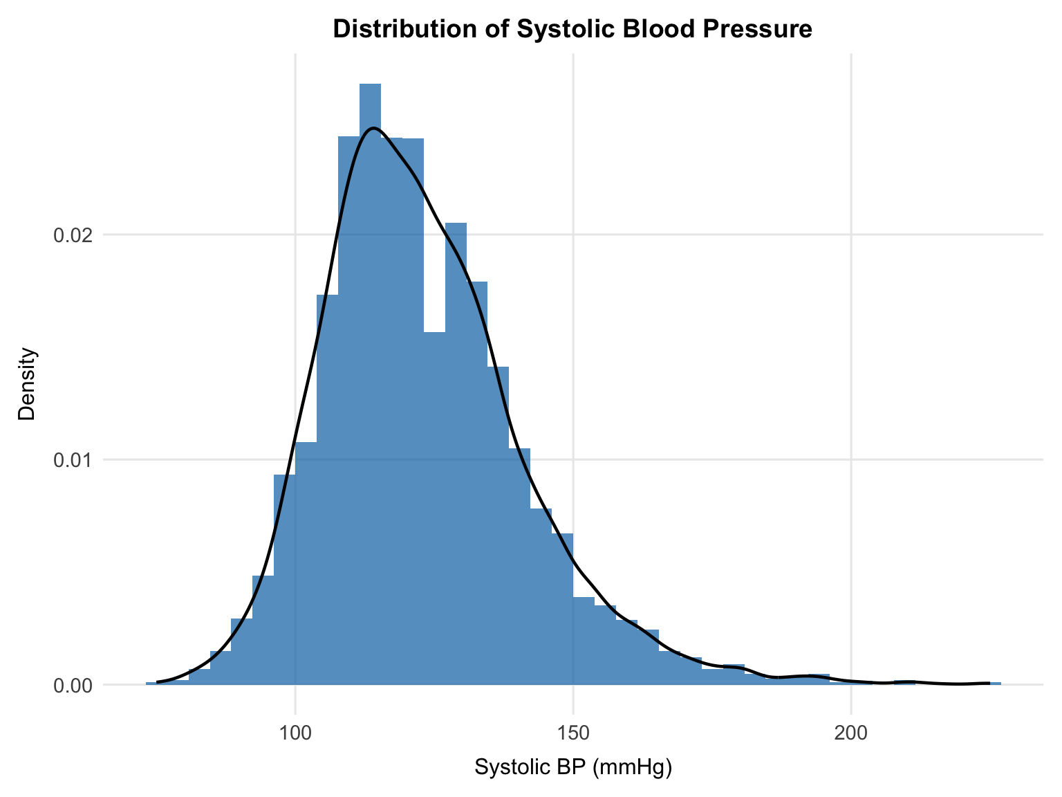
Before modelling, we examine the distribution of the outcome variable. Linear regression assumes approximately normally distributed residuals, so checking the shape of the outcome is a useful first pass to identify any major departures (e.g. skew or multimodality) that might require transformation.
```{r}
#| label: eda-sbp
#| code-summary: "SBP distribution"
ggplot(df_cc, aes(x = sbp)) +
    geom_histogram(aes(y = after_stat(density)), bins = 40,
                fill = palette_epi["blue"], alpha = 0.7) +
    geom_density(linewidth = 0.8) +
    labs(x = "Systolic BP (mmHg)", y = "Density",
        title = "Distribution of Systolic Blood Pressure") +
    theme(plot.title = element_text(hjust = 0.5))
```
SBP is approximately normally distributed with a mild right skew, centred around 120 mmHg. The distribution is unimodal, with a slightly extended upper tail but no obvious multimodality or extreme departure in the tails. Overall, this supports using SBP in its original scale for linear regression.
---
## Physical Activity
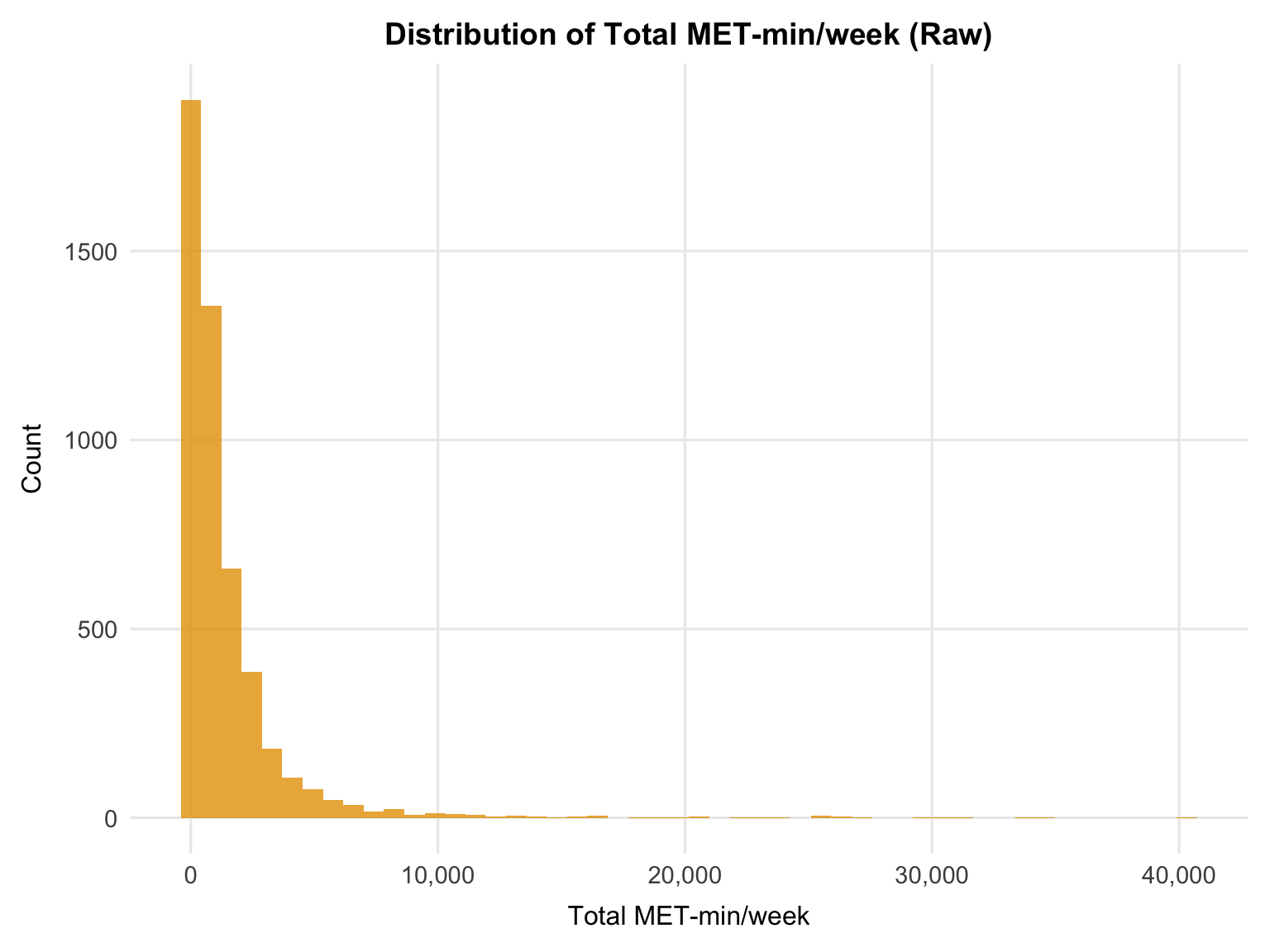
Physical activity is the primary exposure of interest and requires additional preprocessing before modelling. The raw MET variable shows distributional features that make it unsuitable for direct inclusion in a linear regression model.
```{r}
#| label: eda-pa-raw
#| code-summary: "total_met raw distribution - zero inflation"
ggplot(df_cc, aes(x = total_met)) +
    geom_histogram(bins = 50, fill = palette_epi["orange"], alpha = 0.8) +
    scale_x_continuous(labels = scales::comma) +
    labs(x = "Total MET-min/week", y = "Count",
        title = "Distribution of Total MET-min/week (Raw)") +
    theme(plot.title = element_text(hjust = 0.5))
```
The raw distribution is characterised by two key issues: a large spike at zero (participants reporting no leisure physical activity) and pronounced right skew, with a long tail extending beyond 40,000 MET-min/week. Together, these features would likely produce poorly distributed residuals and leverage issues in a linear model if the variable were used untransformed.
```{r}
#| label: eda-pa-log
#| code-summary: "log(total_met + 1) distribution"
ggplot(df_cc, aes(x = log(total_met + 1))) +
    geom_histogram(aes(y = after_stat(density)), bins = 40,
                fill = palette_epi["orange"], alpha = 0.8) +
    geom_density(linewidth = 0.8) +
    labs(x = "log(Total MET-min/week + 1)", y = "Density",
        title = "Distribution of Total MET-min/week (Log-transformed)") +
    theme(plot.title = element_text(hjust = 0.5))
```
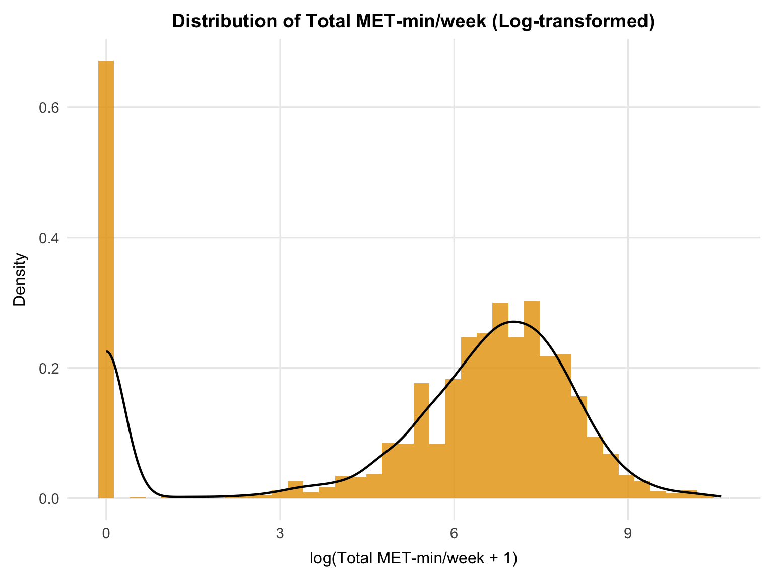
Applying a log transformation (`log(total_met + 1)`) substantially improves the distribution. The transformed variable remains zero-inflated (with `log(0 + 1) = 0`), but the upper tail is compressed, and the distribution becomes more symmetric among active individuals.
The transformed distribution suggests two broad behavioural groups: a large inactive group at zero (approximately 38% of the sample), and a continuous distribution of activity levels among those reporting any exercise. While this can appear bimodal, it primarily reflects the separation between inactivity and varying degrees of activity, rather than two distinct "types" of active individuals.
Based on this, the `log(total_met + 1)` transformation specified in the analysis plan is retained for modelling. For clarity, the transformation is applied inline here for exploration; a dedicated `log_total_met` variable is created during the data wrangling step prior to regression.
---
## Continuous Predictors vs SBP
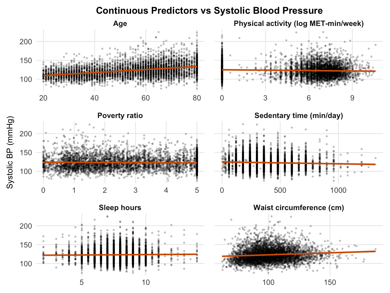
To get an initial sense of the data, we plot each continuous predictor against systolic blood pressure (SBP) with a fitted linear trend. These are unadjusted bivariate relationships, so they are useful for spotting broad patterns, but not for estimating independent effects.
```{r}
#| label: eda-scatter
#| code-summary: "Faceted scatterplots: each continuous predictor vs SBP"
plot_df <- df_cc |>
    mutate(log_total_met = log(total_met + 1)) |>
    select(sbp, age, log_total_met, poverty_ratio,
        sedentary_min_day, sleep_hours, waist_cm) |>
    pivot_longer(
        cols = -sbp,
        names_to = "predictor",
        values_to = "value"
    ) |>
    mutate(
        predictor = factor(predictor,
            levels = c("age", "log_total_met", "poverty_ratio",
                       "sedentary_min_day", "sleep_hours", "waist_cm"),
            labels = c("Age", "Physical activity (log MET-min/week)", "Poverty ratio",
                       "Sedentary time (min/day)", "Sleep hours", "Waist circumference (cm)")
        )
    )

ggplot(plot_df, aes(x = value, y = sbp)) +
    geom_point(alpha = 0.2, size = 0.7) +
    geom_smooth(method = "lm", se = TRUE, color = palette_epi["vermillion"]) +
    facet_wrap(~predictor, scales = "free_x", ncol = 2) +
    labs(x = NULL, y = "Systolic BP (mmHg)",
        title = "Continuous Predictors vs Systolic Blood Pressure") +
    theme(
        plot.title = element_text(hjust = 0.5),
        strip.text = element_text(face = "bold")
    )
```
Age shows the clearest positive association with SBP, which is consistent with the expected increase in blood pressure across the life course. Waist circumference also trends upward, suggesting higher central adiposity is associated with higher SBP. In contrast, log-transformed physical activity and poverty ratio show weak negative associations, with higher activity and higher income tending to correspond to slightly lower SBP, although both relationships are fairly noisy. Sleep duration and sedentary time show little obvious linear pattern in these unadjusted plots. These patterns are descriptive rather than inferential. The multivariable regression model will estimate each association while adjusting for the others.
---
## Categorical Predictors vs SBP
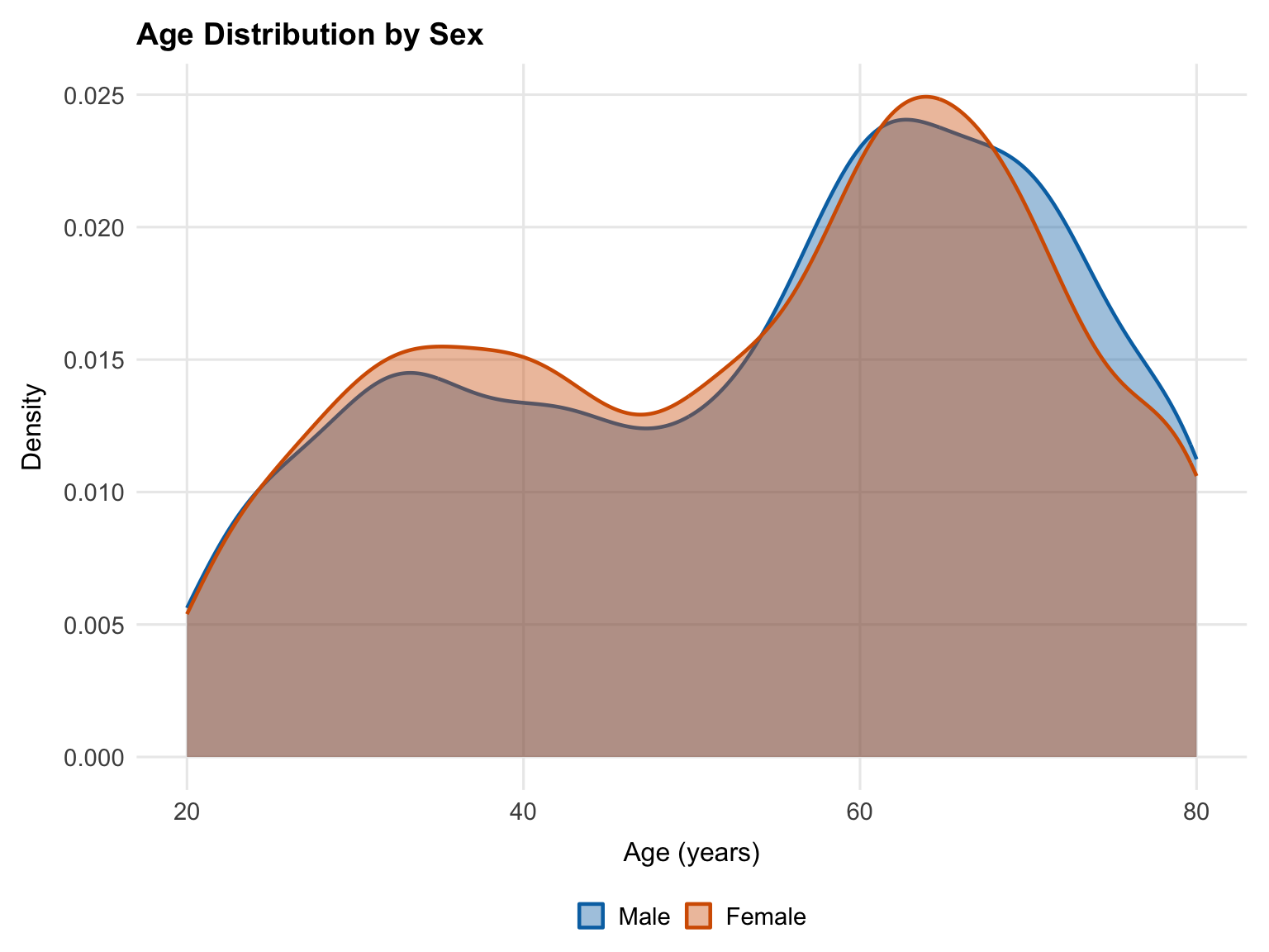
Before interpreting sex differences in SBP, we check whether the two groups are comparably aged. Because SBP rises with age, an age skew between male and female participants could produce or mask a sex effect entirely.
```{r}
#| label: eda-age-by-sex
#| code-summary: "Double density: age distribution by sex"
ggplot(df_cc, aes(x = age, fill = sex, color = sex)) +
    geom_density(alpha = 0.4, linewidth = 0.8) +
    scale_fill_manual(values = unname(palette_epi[c("blue", "vermillion")])) +
    scale_color_manual(values = unname(palette_epi[c("blue", "vermillion")])) +
    labs(x = "Age (years)", y = "Density",
        title = "Age Distribution by Sex",
        fill = NULL, color = NULL)
```
The age distributions for male and female participants are nearly identical, with the same bimodal shape and peaks around 35 and 62 years. Any observed sex difference in SBP is unlikely to be an artifact of differential age composition between groups.
```{r}
#| label: eda-boxplot-sex
#| code-summary: "Boxplot: SBP by sex"
ggplot(df_cc, aes(x = sex, y = sbp, fill = sex)) +
    geom_boxplot(alpha = 0.7, outlier.size = 0.7) +
    scale_fill_epi() +
    labs(x = NULL, y = "Systolic BP (mmHg)", title = "SBP by Sex") +
    theme(legend.position = "none",
        plot.title = element_text(hjust = 0.5))
```
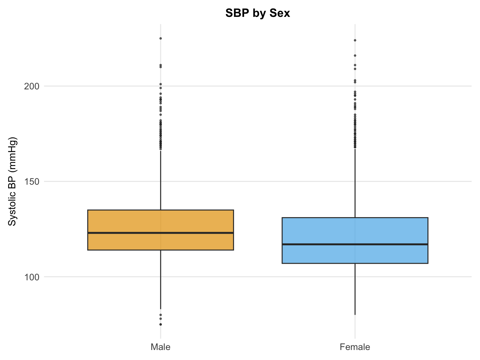
Male participants show a slightly higher median SBP than female participants. Given the near-identical age distributions confirmed above, this difference is unlikely to reflect differential age composition between groups. The association will be estimated more precisely in the adjusted regression model.
```{r}
#| label: eda-boxplot-race
#| code-summary: "Boxplot: SBP by race"
ggplot(df_cc, aes(x = sbp, y = race, fill = race)) +
    geom_boxplot(alpha = 0.7, outlier.size = 0.7) +
    scale_fill_epi() +
    labs(x = "Systolic BP (mmHg)", y = NULL, title = "SBP by Race") +
    theme(legend.position = "none",
        plot.title = element_text(hjust = 0.5))
```
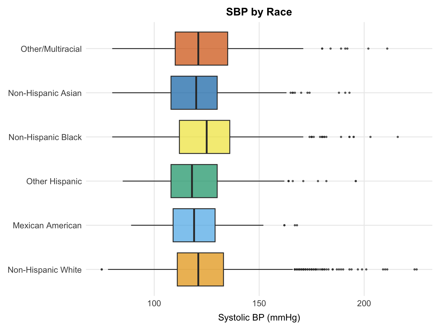
Non-Hispanic Black participants have the highest median SBP, followed by Non-Hispanic White and Other Hispanic groups, while Non-Hispanic Asian participants show the lowest median SBP. These patterns are consistent with well-documented racial disparities in hypertension prevalence in the United States. As with the other plots in this section, these are unadjusted comparisons: differences in age, socioeconomic status, and other covariates may explain part of the observed variation.
```{r}
#| label: eda-boxplot-education
#| code-summary: "Boxplot: SBP by education"
ggplot(df_cc, aes(x = sbp, y = education, fill = education)) +
    geom_boxplot(alpha = 0.7, outlier.size = 0.7) +
    scale_fill_epi() +
    labs(x = "Systolic BP (mmHg)", y = NULL, title = "SBP by Education") +
    theme(legend.position = "none",
          plot.title = element_text(hjust = 0.5))
```
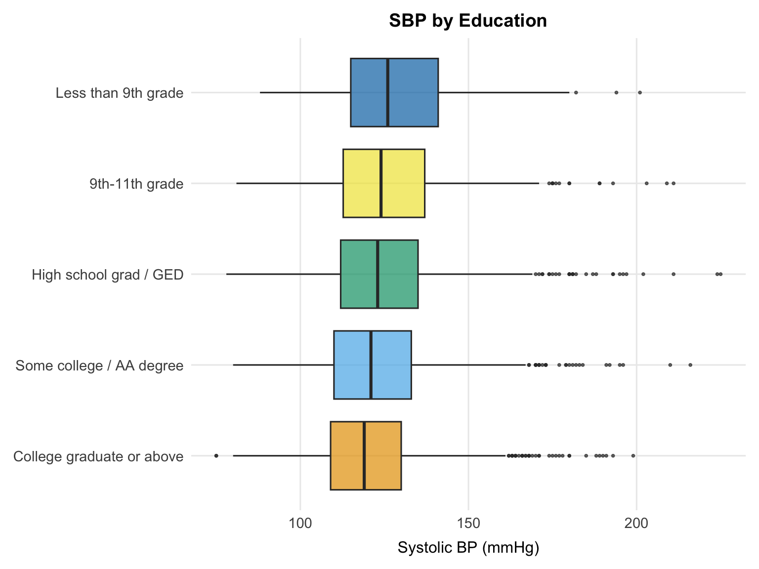
A modest inverse gradient is visible, with lower education levels tending toward higher median SBP. The difference is most pronounced between the college graduate group and those with less than a high school education, which is consistent with the broader literature linking educational attainment to cardiovascular risk through pathways such as health literacy, occupational exposures, and access to care. As with the other categorical plots, this is an unadjusted comparison and the pattern may shift once age and other socioeconomic variables are accounted for in the regression model.
```{r}
#| label: eda-boxplot-smoking
#| code-summary: "Boxplot: SBP by smoking status"
ggplot(df_cc, aes(x = smoking_status, y = sbp, fill = smoking_status)) +
    geom_boxplot(alpha = 0.7, outlier.size = 0.7) +
    scale_fill_manual(values = unname(palette_epi[c("blue", "orange", "vermillion")])) +
    labs(x = NULL, y = "Systolic BP (mmHg)", title = "SBP by Smoking Status") +
    theme(legend.position = "none",
        plot.title = element_text(hjust = 0.5))
```
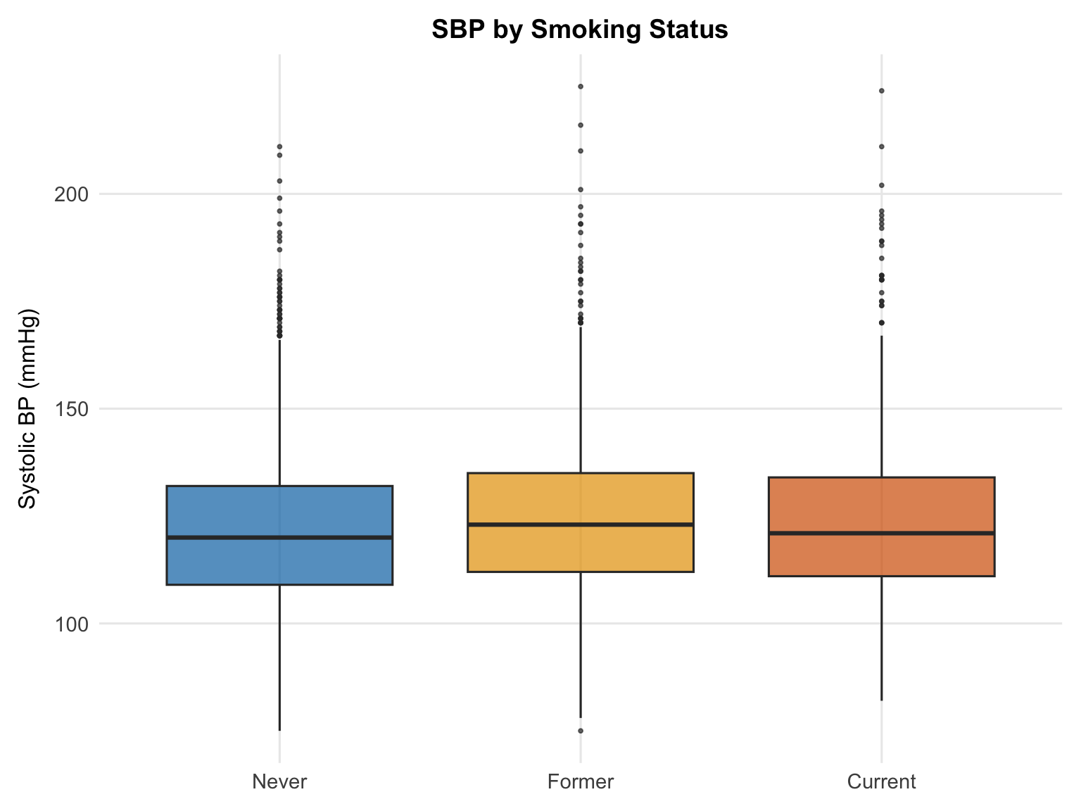
Former smokers have a higher median SBP than both current and never smokers, a counterintuitive pattern that likely reflects confounding by age. Former smokers tend to be older on average, and age is strongly associated with higher SBP. This is a good example of how unadjusted comparisons can be misleading: the apparent "former smoker effect" may attenuate or disappear once age is accounted for in the regression model.
```{r}
#| label: eda-boxplot-food-security
#| code-summary: "Boxplot: SBP by food security"
ggplot(df_cc, aes(x = sbp, y = food_security, fill = food_security)) +
    geom_boxplot(alpha = 0.7, outlier.size = 0.7) +
    scale_fill_epi() +
    labs(x = "Systolic BP (mmHg)", y = NULL, title = "SBP by Food Security") +
    theme(legend.position = "none",
        plot.title = element_text(hjust = 0.5))
```
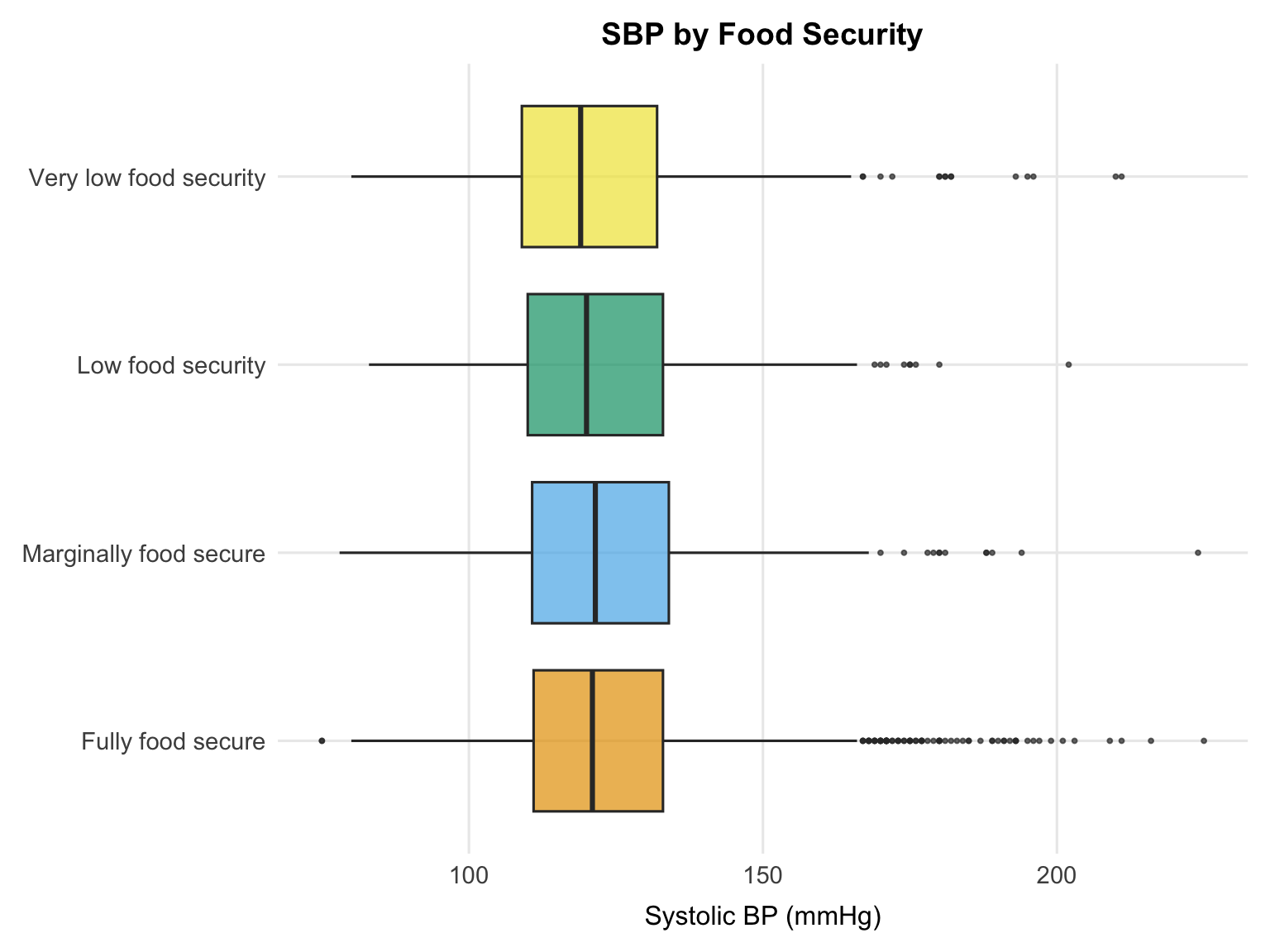
The food security plot shows a modest gradient, with fully food secure participants tending to have slightly lower median SBP. However, there is substantial overlap across categories, and differences in medians are small. Food security likely operates through indirect pathways such as stress, diet quality, and access to healthcare, so a strong unadjusted association is not necessarily expected.
```{r}
#| label: eda-boxplot-diabetes
#| code-summary: "Boxplot: SBP by diabetes status"
ggplot(df_cc, aes(x = diabetes_flag, y = sbp, fill = diabetes_flag)) +
    geom_boxplot(alpha = 0.7, outlier.size = 0.7) +
    scale_fill_manual(values = unname(palette_epi[c("blue", "vermillion")])) +
    labs(x = NULL, y = "Systolic BP (mmHg)", title = "SBP by Diabetes Status") +
    theme(legend.position = "none",
        plot.title = element_text(hjust = 0.5))
```
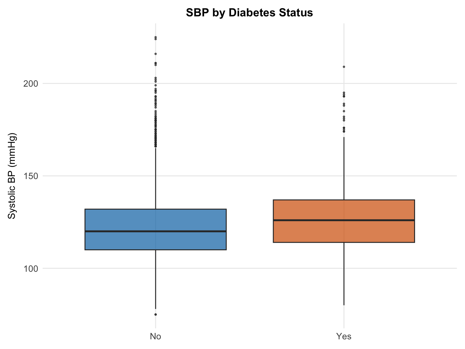
Participants with diabetes have a slightly higher median SBP than those without, consistent with the well-established relationship between diabetes and hypertension. These conditions share underlying mechanisms, including insulin resistance, endothelial dysfunction, and increased arterial stiffness. The difference in medians is modest in the unadjusted plot, though the association may become more pronounced after adjusting for other covariates in the regression model.
---
## Correlation Matrix
We examine pairwise correlations among the continuous variables to assess potential multicollinearity. High correlations between predictors can inflate standard errors and destabilise coefficient estimates in regression models.
```{r}
#| label: eda-pairs
#| code-summary: "Pairwise correlations among continuous model variables"
#| fig-width: 12
#| fig-height: 10
df_cc |>
    mutate(log_total_met = log(total_met + 1)) |>
    select(sbp, age, waist_cm, poverty_ratio, sleep_hours,
        sedentary_min_day, log_total_met) |>
    rename(
        "Systolic BP (mmHg)"                   = sbp,
        "Age (years)"                          = age,
        "Waist circumference (cm)"             = waist_cm,
        "Poverty-income ratio"                 = poverty_ratio,
        "Sleep hours"                          = sleep_hours,
        "Sedentary time (min/day)"             = sedentary_min_day,
        "Physical activity (log MET-min/week)" = log_total_met
    ) |>
    ggpairs(
    upper = list(continuous = wrap("cor", size = 3.5)),
    lower = list(continuous = wrap("points", alpha = 0.2, size = 0.5)),
    diag  = list(continuous = wrap("densityDiag"))
    ) +
    theme_epi(base_size = 10)
```
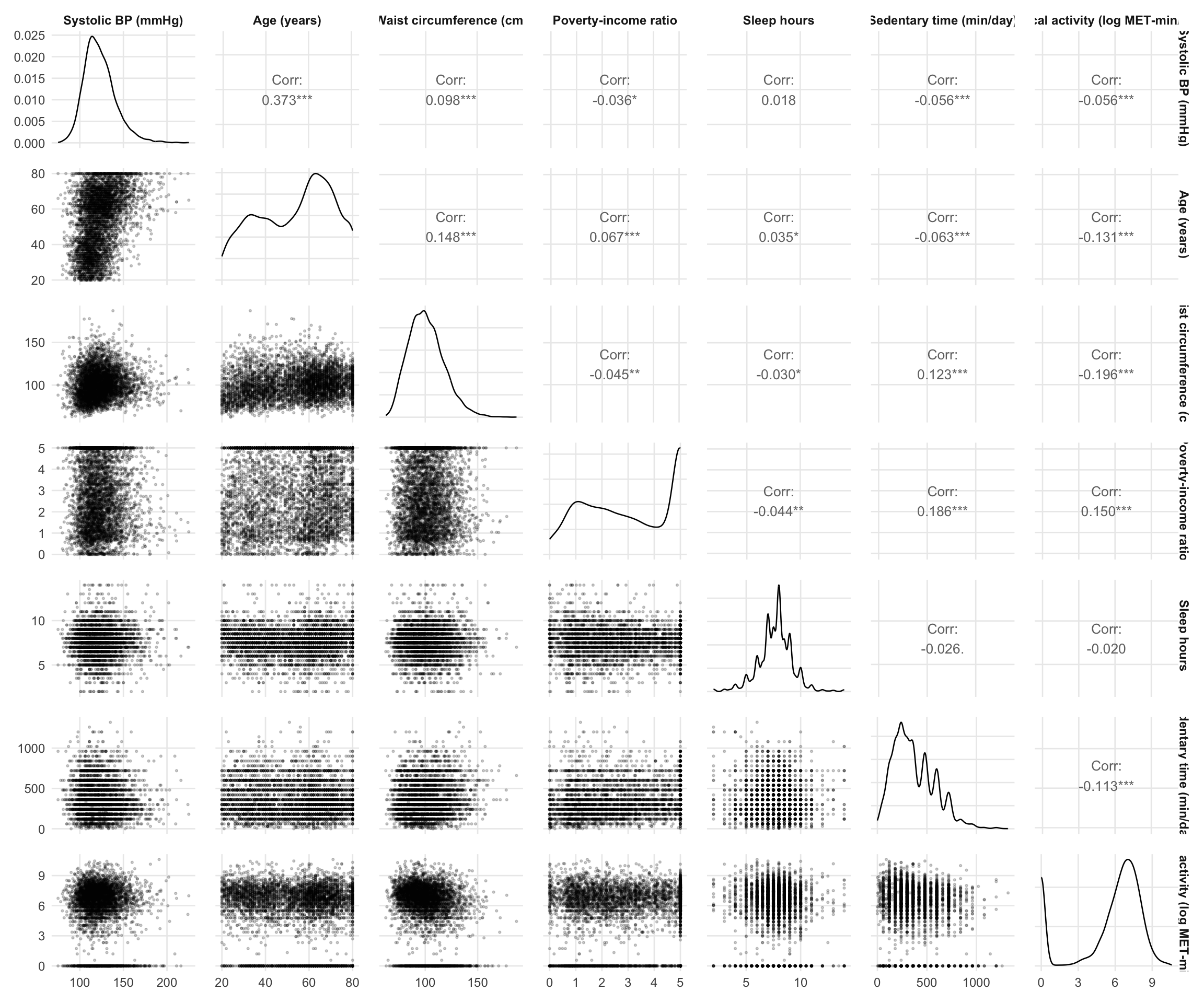
Age shows the strongest positive correlation with SBP (r = 0.373), followed by waist circumference (r = 0.098). Other associations with SBP are weak in magnitude: poverty ratio (r = -0.036), sedentary time and log physical activity are each r = -0.056, and sleep hours is essentially uncorrelated (r = 0.018).
Among predictors, the strongest correlation is between waist circumference and log physical activity (r = -0.196), followed by poverty ratio and sedentary time (r = 0.186), and age and log physical activity (r = -0.131). The waist-activity and poverty-sedentary relationships are directionally consistent with expected behavioural and socioeconomic patterns, though their magnitude is modest.
No pair of predictors shows a correlation of sufficient magnitude to raise concerns about multicollinearity. All correlations are well below conventional thresholds (e.g. |r| ≥ 0.7), suggesting that the model should be stable from a collinearity perspective.
---
## EDA Summary
The outcome (SBP) is approximately normally distributed, supporting its use on the original scale in linear regression. Age and waist circumference show the strongest positive unadjusted associations with SBP, while physical activity and socioeconomic indicators demonstrate weaker unadjusted associations with SBP.
The physical activity variable required transformation due to zero inflation and right skew; a `log(total_met + 1)` specification improves its distribution and is retained for modelling. Several categorical variables (e.g. smoking status, food security) show modest unadjusted differences, with patterns suggestive of confounding, particularly by age.
Missingness is low overall, with complete case analysis retaining ~83% of observations. Correlations between predictors are modest, with no evidence of problematic multicollinearity.
Taken together, the data are well-suited for multivariable linear regression, which will allow these relationships to be estimated while adjusting for confounding, in the regression notebook that follows.
---
## Session Info
```{r}
#| label: session-info
#| collapse: true
#| code-summary: "R session info"
sessionInfo()
```