---
title: "Multiple Linear Regression"
subtitle: "{{< var study_title >}}"
---
## Setup
The below packages are loaded for this analysis. `arrow` reads the parquet mart, `gtsummary` produces the regression tables, `broom` extracts model fit statistics, `car` provides variance inflation factors, and `performance` with `see` power the `check_model()` diagnostic panel. A custom plot theme and colour palette are sourced from `R/plot_theme.R`.
```{r}
#| label: setup
#| collapse: true
#| code-summary: "Load packages and helpers"
library(here)
library(tidyverse)
library(arrow)
library(gtsummary)
library(broom)
library(car)
library(performance)
library(see)
library(patchwork)
library(cowplot)

source(here("R", "plot_theme.R")) # palette_epi, theme_epi(), scale_*_epi()
```
---
## Data Import & Preparation
We apply the same wrangling pipeline used in the EDA notebook: sentinel-value recodes, MET derivation, factor recodes, and a complete case filter restricted to the outcome and 12 predictors. A `log_total_met` column is added here so the transformation is explicit in the data frame and referenced by name in the model formula.
```{r}
#| label: import
#| code-summary: "Read parquet mart, apply wrangling, complete case filter"
df_raw <- read_parquet(here("data", "processed", "analysis_dataset.parquet"))

# Derived variables: MET score and log transform
# NHANES uses 7777 (refused) and 9999 (don't know) as sentinel values;
# recode to NA before any arithmetic to avoid inflated activity estimates
df <- df_raw |>
    mutate(
        mod_min_session   = if_else(mod_min_session   %in% c(7777, 9999), NA_real_, mod_min_session),
        vig_min_session   = if_else(vig_min_session   %in% c(7777, 9999), NA_real_, vig_min_session),
        vig_freq          = if_else(vig_freq          %in% c(7777, 9999), NA_real_, vig_freq),
        sedentary_min_day = if_else(sedentary_min_day %in% c(7777, 9999), NA_real_, sedentary_min_day),
        # NHANES records frequency in varying units; convert all to per-week
        mod_freq_per_week = case_when(
            mod_freq_unit == "D" ~ mod_freq * 7,
            mod_freq_unit == "W" ~ mod_freq,
            mod_freq_unit == "M" ~ mod_freq / 4.3,
            mod_freq_unit == "Y" ~ mod_freq / 52,
            TRUE                 ~ NA_real_
        ),
        vig_freq_per_week = case_when(
            vig_freq_unit == "D" ~ vig_freq * 7,
            vig_freq_unit == "W" ~ vig_freq,
            vig_freq_unit == "M" ~ vig_freq / 4.3,
            vig_freq_unit == "Y" ~ vig_freq / 52,
            TRUE                 ~ NA_real_
        ),
        # MET-min/week: moderate = 4 METs, vigorous = 8 METs (standard multipliers);
        # coalesce to 0 so participants with no reported activity aren't dropped
        mod_met     = coalesce(mod_freq_per_week * mod_min_session, 0) * 4,
        vig_met     = coalesce(vig_freq_per_week * vig_min_session, 0) * 8,
        total_met   = mod_met + vig_met,
        # +1 before log to handle zero-activity participants without producing -Inf
        log_total_met = log(total_met + 1)
    )

# Factor recodes: set reference levels to align with model interpretation
df <- df |>
    mutate(
        sex = factor(
            case_when(sex_raw == 1 ~ "Male", sex_raw == 2 ~ "Female"),
            levels = c("Male", "Female")
        ),
        race = factor(
            case_when(
                race_raw == 1 ~ "Mexican American",
                race_raw == 2 ~ "Other Hispanic",
                race_raw == 3 ~ "Non-Hispanic White",
                race_raw == 4 ~ "Non-Hispanic Black",
                race_raw == 6 ~ "Non-Hispanic Asian",
                race_raw == 7 ~ "Other/Multiracial"
            ),
            levels = c(
                "Non-Hispanic White", "Mexican American", "Other Hispanic",
                "Non-Hispanic Black", "Non-Hispanic Asian", "Other/Multiracial"
            )
        ),
        education = factor(
            case_when(
                education_raw == 1         ~ "Less than 9th grade",
                education_raw == 2         ~ "9th-11th grade",
                education_raw == 3         ~ "High school grad / GED",
                education_raw == 4         ~ "Some college / AA degree",
                education_raw == 5         ~ "College graduate or above",
                education_raw %in% c(7, 9) ~ NA_character_
            ),
            levels = c(
                "College graduate or above", "Some college / AA degree",
                "High school grad / GED", "9th-11th grade", "Less than 9th grade"
            )
        ),
        smoking_status = factor(
            case_when(
                ever_smoked == 2                            ~ "Never",
                ever_smoked == 1 & current_smoker == 3     ~ "Former",
                ever_smoked == 1 & current_smoker %in% c(1, 2) ~ "Current",
                TRUE                                        ~ NA_character_
            ),
            levels = c("Never", "Former", "Current")
        ),
        food_security = factor(
            case_when(
                food_security_raw == 1 ~ "Fully food secure",
                food_security_raw == 2 ~ "Marginally food secure",
                food_security_raw == 3 ~ "Low food security",
                food_security_raw == 4 ~ "Very low food security"
            ),
            levels = c(
                "Fully food secure", "Marginally food secure",
                "Low food security", "Very low food security"
            )
        ),
        diabetes_flag = factor(
            case_when(
                diabetes_diagnosis == 1         ~ "Yes",
                diabetes_diagnosis %in% c(2, 3) ~ "No",
                diabetes_diagnosis %in% c(7, 9) ~ NA_character_
            ),
            levels = c("No", "Yes")
        ),
        poverty_ratio = poverty_raw
    )

# Complete case filter: restrict to outcome + 12 predictors + survey design vars;
# drop_na is scoped to model_vars only so unrelated missingness doesn't reduce n
model_vars <- c(
    "sbp", "log_total_met", "sedentary_min_day", "age", "sex", "race",
    "education", "waist_cm", "poverty_ratio", "sleep_hours", "smoking_status",
    "food_security", "diabetes_flag"
)

df_cc <- df |>
    drop_na(all_of(model_vars)) |>
    select(id, all_of(model_vars), mec_weight, psu, strata)

cat(sprintf("Original n:      %d\nComplete case n: %d\nExcluded:        %d\n",
            nrow(df), nrow(df_cc), nrow(df) - nrow(df_cc)))
```
The wrangling pipeline is identical to the EDA. The one addition is `log_total_met = log(total_met + 1)`, which is included in `model_vars` in place of the raw `total_met`. This ensures the complete case filter operates on the transformed variable that enters the model. The final sample size after complete case filtering is `r nrow(df_cc)`. The number of excluded observations (n = `r nrow(df) - nrow(df_cc)`) is not negligible, but the complete case approach is justified by the EDA's missingness analysis: no variable has >10% missing, and missingness is plausibly random conditional on observed covariates (e.g. education, poverty ratio). Multiple imputation would be an alternative strategy if we had stronger evidence of systematic missingness or wanted to retain a larger sample size.
---
## Model
We fit two nested models to assess whether SDoH and lifestyle factors explain variance in SBP beyond basic demographic characteristics.
### Base model
The base model includes only non-modifiable demographic predictors: age, sex, and race/ethnicity. This serves as the reference against which the explanatory contribution of social determinants of health (SDoH) variables are evaluated.
```{r}
#| label: model-formula-base
#| code-summary: "Define base model formula"
model_formula_base <- sbp ~ age + sex + race
```
```{r}
#| label: model-fit-base
#| code-summary: "Fit base model"
model_base <- lm(model_formula_base, data = df_cc)
```
### Full model
The full model adds the SDoH and lifestyle predictors to the demographic base: physical activity, sedentary time, waist circumference, education, poverty-income ratio, sleep, smoking status, food security, and diabetes status.
```{r}
#| label: model-formula-full
#| code-summary: "Define full model formula"
model_formula_full <- sbp ~ age + sex + race +
    log_total_met + sedentary_min_day + waist_cm +
    education + poverty_ratio + sleep_hours +
    smoking_status + food_security + diabetes_flag
```
```{r}
#| label: model-fit-full
#| code-summary: "Fit full model"
model <- lm(model_formula_full, data = df_cc)
```
Physical activity enters as `log_total_met`, the `log(total_met + 1)` transformation justified in the EDA by the variable's zero inflation and right skew. All other continuous predictors enter untransformed. Reference levels are set by factor level ordering applied during wrangling: Male (sex), Non-Hispanic White (race), College graduate or above (education), Never (smoking), Fully food secure (food security), No diabetes (diabetes).
---
## Diagnostics
Before interpreting the model estimates, we assess whether the assumptions underlying OLS regression hold. Violations, particularly multicollinearity, non-constant variance, or influential observations, can distort coefficients and standard errors, undermining the validity of inference. We proceed in three steps: first checking for multicollinearity via variance inflation factors, then evaluating residual behavior through a standard diagnostic panel, and finally identifying and characterizing any observations with undue influence on the model.
### Multicollinearity
Multicollinearity occurs when predictors are highly correlated with one another, making it difficult for the model to isolate each predictor's independent contribution to the outcome. In practice, this inflates standard errors and destabilizes coefficient estimates: a predictor may appear non-significant not because it lacks a relationship with SBP, but because its variance is shared with another predictor. We use variance inflation factors (VIF) to detect this: values above √5 ≈ 2.24 (on the GVIF scale used for categorical predictors) would signal a concern. Given the EDA showed no predictor pair with |r| ≥ 0.7, we expect all predictors to be well within this threshold.
```{r}
#| label: diag-vif
#| code-summary: "Variance inflation factors (numeric)"
vif(model)
```
Because the model contains multi-level categorical predictors, `car::vif()` returns Generalised VIF (GVIF). The relevant column for interpretation is `GVIF^(1/(2*Df))`, which is analogous to √VIF.
All `GVIF^(1/(2*Df))` values were well below the 2.24 threshold, with the highest observed for `poverty_ratio` (1.30) and `age` (1.10). Education and poverty-income ratio, the predictor pair most likely to share variance given both capture socioeconomic position, showed no evidence of collinearity (1.07 and 1.30 respectively). Multicollinearity is not a concern in this model.
```{r}
#| label: diag-combined
#| code-summary: "Diagnostic panel: collinearity + residual checks (3×2 patchwork)"
#| fig-width: 12
#| fig-height: 12
#| warning: false
#| fig-keep: last
# Shared theme applied to all six panels: centred titles/subtitles and
# consistent plot margins
diag_theme <- theme(
  plot.title    = element_text(hjust = 0.5, margin = margin(b = 1)),
  plot.subtitle = element_text(hjust = 0.5, margin = margin(t = 1)),
  plot.margin   = margin(t = 12, r = 5, b = 12, l = 5)
)

# VIF collinearity plot: legend removed (all predictors in safe zone),
# labels shortened to reduce 45° axis footprint
cc_plot <- plot(check_collinearity(model)) +
  scale_x_discrete(labels = c(
    age               = "Age",
    diabetes_flag     = "Diabetes",
    education         = "Education",
    food_security     = "Food security",
    log_total_met     = "PA (log MET)",
    poverty_ratio     = "PIR",
    race              = "Race/eth.",
    sedentary_min_day = "Sedentary time",
    sex               = "Sex",
    sleep_hours       = "Sleep hours",
    smoking_status    = "Smoking status",
    waist_cm          = "Waist circ."
  )) +
  labs(y = "Variance Inflation\nFactor (VIF, log-scale)") +
  diag_theme +
  theme(
    axis.text.x = element_text(angle = 45, hjust = 1, vjust = 1, size = 8),
    legend.position = "none"
  )

# Run all five check_model diagnostics in one call; results indexed as a list
cm_plots <- plot(check_model(
  model,
  check = c("pp_check", "linearity", "homogeneity", "outliers", "qq")
))

# PPC: see's subtitle hjust ignores theme overrides, so we suppress the native
# x-axis title and redraw it via cowplot's draw_label at a fixed position
pp_inner <- cm_plots[[1]] +
  labs(x = NULL) +
  diag_theme +
  theme(
    legend.position = c(0.82, 0.82),
    axis.title.x    = element_blank(),
    plot.margin     = margin(t = 12, r = 5, b = 24, l = 5)
  )

pp_plot <- wrap_elements(
  full = ggdraw() +
    draw_plot(pp_inner, x = 0, y = 0, width = 1, height = 1) +
    draw_label(
      "SBP (mmHg)",
      x = 0.5, y = 0.035,
      hjust = 0.5, vjust = 0,
      size = 10
    )
)

# Remaining four diagnostics get diag_theme applied; QQ y-axis label corrected
lin_plot <- cm_plots[[2]] + diag_theme
hom_plot <- cm_plots[[3]] + diag_theme
out_plot <- cm_plots[[4]] + diag_theme
qq_plot  <- cm_plots[[5]] + labs(y = "Sample Quantiles") + diag_theme

# Assemble 3×2 patchwork; cc_plot and pp_plot wrapped equally to equalise
# space allocation in the top row
((cc_plot | pp_plot) + plot_layout(widths = c(1, 1))) /
(lin_plot | hom_plot) /
(out_plot | qq_plot)
```
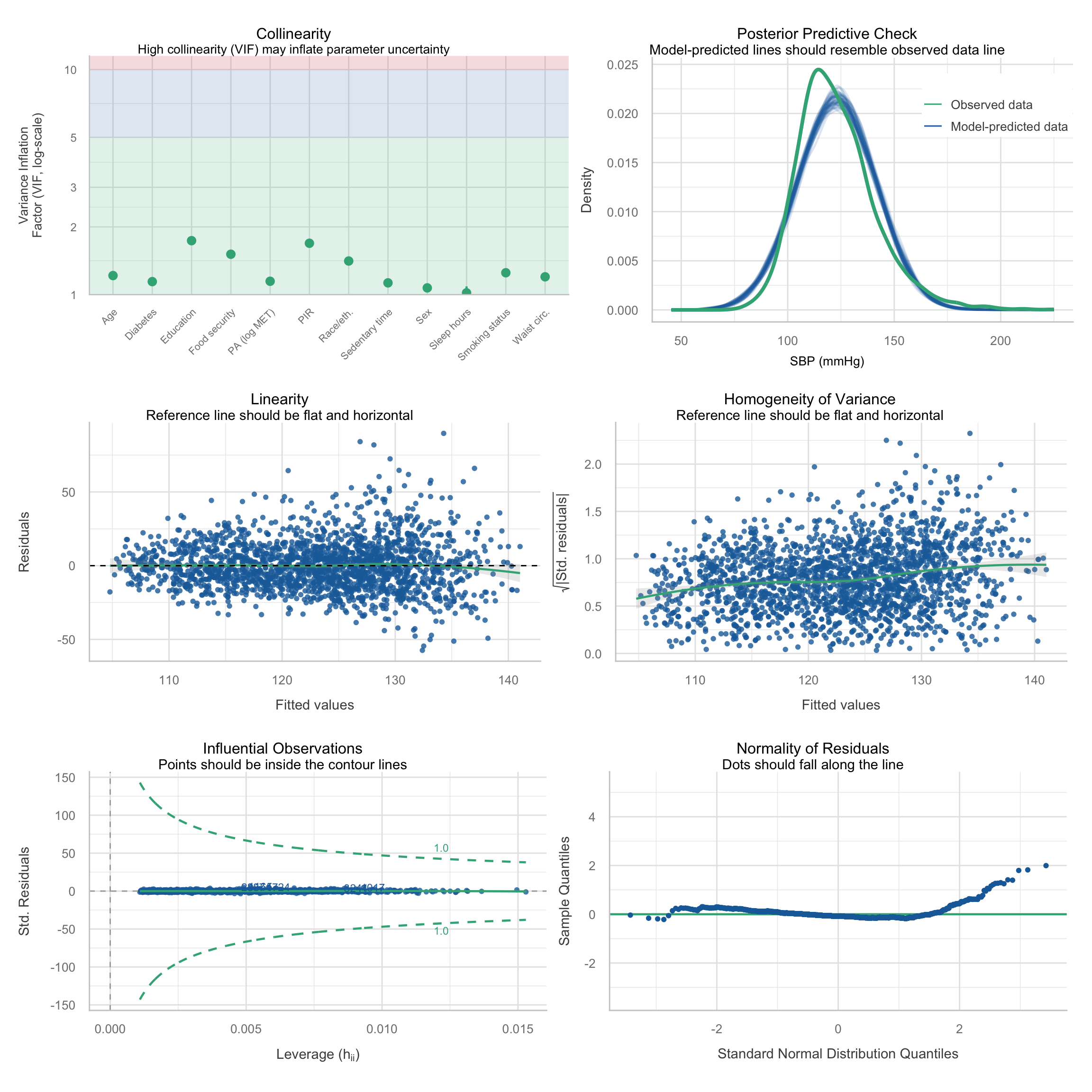
The diagnostic panel presents six checks in a 3×2 grid: (1) **collinearity**, GVIF values for each predictor, with the threshold at √5 ≈ 2.24; (2) **posterior predictive check**, model-predicted distribution should resemble the observed SBP distribution; (3) **linearity**, residuals vs fitted values should show no systematic curvature; (4) **homogeneity of variance**, spread of standardised residuals should be consistent across fitted values; (5) **influential observations**, points should fall within Cook's distance contours; (6) **normality of residuals**, the Q-Q plot should track the reference line.
The posterior predictive check showed good agreement between the model-predicted and observed SBP distributions. The linearity and homogeneity of variance plots showed no systematic patterns, supporting both assumptions. The Q-Q plot tracked the reference line well through the bulk of the distribution, with moderate tail departures consistent with the mild right skew typical of SBP data; with n = `r nrow(df_cc)`, this is unlikely to meaningfully affect inference. The influential observations panel flagged a small number of extreme residuals, investigated below.
### Influential observations
```{r}
#| label: diag-outliers
#| code-summary: "Identify observations with |standardised residual| > 3"
augment(model, data = df_cc) |>
    filter(abs(.std.resid) > 3) |>
    select(id, sbp, .fitted, .resid, .std.resid, .hat, .cooksd) |>
    arrange(desc(abs(.std.resid)))
```
Fifty-nine observations (1.2% of the sample) had |standardised residual| > 3. Under strict normality approximately 15 would be expected (0.3%), so the excess is modest and consistent with the tail departures seen in the Q-Q plot. Critically, Cook's distances for all 59 observations were negligible (maximum 0.008), confirming that no single observation has undue influence on the coefficient estimates. The flagged observations fall into two groups: individuals with elevated SBP (167-225 mmHg) whose values the model underpredicts (plausibly reflecting uncontrolled hypertension absent a medication covariate), and a smaller group with very low SBP (75-87 mmHg) despite covariate profiles that predict elevated values, which may reflect measurement error or recently treated hypertension. No observations were removed; given the negligible Cook's distances, the model estimates are considered robust.
---
## Results
Results are presented in three parts: model comparison to quantify the incremental contribution of SDoH predictors, followed by univariable and multivariable coefficient tables.
### Model comparison
We compare the demographic base model against the full SDoH model using a nested F-test and fit statistics to quantify how much additional variance in SBP is explained by the SDoH and lifestyle predictors.
```{r}
#| label: results-model-comparison-anova
#| code-summary: "F-test: base vs full model"
anova(model_base, model)
```
The nested F-test was highly significant (F(15, 4853) = 3.59, p < 0.001), indicating the SDoH and lifestyle predictors collectively explain a statistically significant increment of variance beyond basic demographics.
```{r}
#| label: results-model-comparison-fit
#| code-summary: "R², adjusted R², AIC, BIC, and n - base vs full model"
tibble(
    model_name = c("Base (age + sex + race)", "Full (+ SDoH & lifestyle)"),
    r_squared  = c(summary(model_base)$r.squared, summary(model)$r.squared),
    adj_r_sq   = c(summary(model_base)$adj.r.squared, summary(model)$adj.r.squared),
    sigma      = c(summary(model_base)$sigma, summary(model)$sigma),
    AIC        = c(AIC(model_base), AIC(model)),
    BIC        = c(BIC(model_base), BIC(model)),
    nobs       = c(nobs(model_base), nobs(model))
) |>
    mutate(delta_r_sq = r_squared - first(r_squared)) |>
    mutate(across(where(is.numeric), \(x) round(x, 3)))
```
The gain in explanatory power was modest: ΔR² = 0.009, meaning the full model accounts for only 0.9 percentage points more variance in SBP than the base model (17.5% vs 16.5%). The residual standard error improved marginally (σ = 16.65 vs 16.71 mmHg). AIC favoured the full model (ΔAIC = -24), but BIC favoured the base model (ΔBIC = +74), reflecting BIC's heavier per-parameter penalty against a model that adds 15 degrees of freedom for a small R² gain. Taken together, the SDoH variables are jointly significant but explain limited incremental variance in SBP in this cross-sectional sample, a finding that likely reflects both the dominant role of age as a predictor and the absence of antihypertensive medication data, which would substantially reduce residual variance.
### Univariable coefficients
```{r}
#| label: results-univariable
#| code-summary: "tbl_uvregression - each predictor unadjusted"
df_cc |>
    select(sbp, log_total_met, sedentary_min_day, age, sex, race,
           education, waist_cm, poverty_ratio, sleep_hours, smoking_status,
           food_security, diabetes_flag) |>
    tbl_uvregression(
        method = lm,
        y = sbp,
        label = list(
            log_total_met     ~ "Physical activity (log MET-min/week)",
            sedentary_min_day ~ "Sedentary time (min/day)",
            age               ~ "Age (years)",
            sex               ~ "Sex",
            race              ~ "Race/ethnicity",
            education         ~ "Education",
            waist_cm          ~ "Waist circumference (cm)",
            poverty_ratio     ~ "Poverty-income ratio",
            sleep_hours       ~ "Sleep hours (weekdays)",
            smoking_status    ~ "Smoking status",
            food_security     ~ "Food security",
            diabetes_flag     ~ "Diabetes"
        )
    ) |>
    bold_labels() |>
    bold_p(t = 0.05) |>
    modify_caption("**Table 2.** Univariable regressions: each predictor vs systolic blood pressure (n = `r nrow(df_cc)`)")
```
The table below shows each predictor's unadjusted association with SBP. Comparing these crude estimates to the adjusted coefficients that follow reveals where confounding, particularly by age, is shaping the apparent relationships.
In crude analysis, age was the strongest continuous predictor (β = 0.40 mmHg per year, 95% CI: 0.37-0.43). Female sex was associated with lower SBP (β = -5.0 mmHg), and Non-Hispanic Black participants had significantly higher crude SBP than Non-Hispanic White participants (β = +3.9 mmHg). Education showed a clear monotonic gradient: each step below college graduate was associated with progressively higher SBP, reaching +8.2 mmHg for those with less than 9th grade education, the strongest SDoH signal in the crude analysis. Diabetes (β = +4.8 mmHg) and waist circumference (β = +0.11 mmHg/cm) were also significantly associated. Physical activity was inversely associated with SBP (β = -0.36 per log MET-min/week). Sedentary time was statistically significant but the per-minute coefficient rounds to zero, reflecting the small unit scale. Sleep hours and food security showed no significant crude associations. Smoking status warrants attention: former and current smokers showed nearly identical crude estimates (+3.3 and +3.0 mmHg respectively), consistent with age confounding, since former smokers are older on average, compressing the crude difference between groups.
### Multivariable coefficients
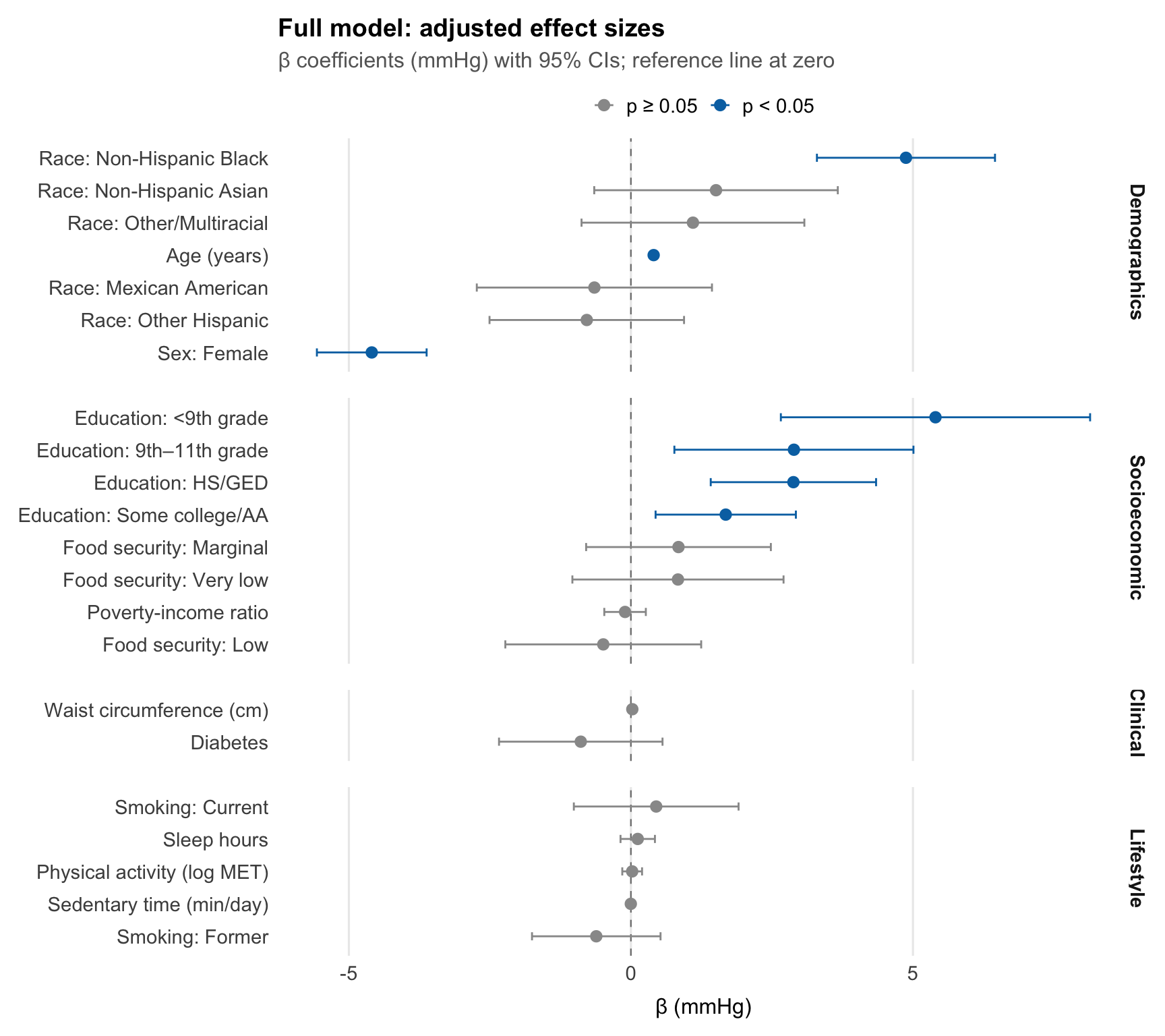
Table 3 presents the adjusted coefficients from the full model, with all predictors entered simultaneously. Estimates reflect each variable's independent association with SBP after accounting for the others.
```{r}
#| label: results-table
#| code-summary: "tbl_regression - adjusted coefficients"
model |>
    tbl_regression(
        label = list(
            log_total_met     ~ "Physical activity (log MET-min/week)",
            sedentary_min_day ~ "Sedentary time (min/day)",
            age               ~ "Age (years)",
            sex               ~ "Sex",
            race              ~ "Race/ethnicity",
            education         ~ "Education",
            waist_cm          ~ "Waist circumference (cm)",
            poverty_ratio     ~ "Poverty-income ratio",
            sleep_hours       ~ "Sleep hours (weekdays)",
            smoking_status    ~ "Smoking status",
            food_security     ~ "Food security",
            diabetes_flag     ~ "Diabetes"
        ),
        intercept = FALSE
    ) |>
    bold_labels() |>
    bold_p(t = 0.05) |>
    modify_caption("**Table 3.** Multivariable linear regression: predictors of systolic blood pressure (n = `r nrow(df_cc)`)")
```
After mutual adjustment, four predictors remained statistically significant: age, sex, Non-Hispanic Black race/ethnicity, and education. Age was the dominant predictor (β = 0.40 mmHg per year, 95% CI: 0.37-0.43), with an estimate identical to the crude, indicating that its association with SBP is not confounded by the other variables in the model. Female sex was associated with 4.6 mmHg lower SBP than male (95% CI: -5.6, -3.6). Non-Hispanic Black participants had 4.9 mmHg higher SBP than Non-Hispanic White participants (95% CI: 3.3-6.5), a disparity that strengthened slightly after adjustment (crude: +3.9 mmHg), suggesting the SDoH variables in this model do not account for the racial disparity in SBP. Non-Hispanic Asian participants showed a sign reversal after adjustment (crude: -1.3 mmHg; adjusted: +1.5 mmHg), though the estimate remained non-significant in both models. Education retained a monotonic gradient: relative to college graduates, SBP was 1.7, 2.9, 2.9, and 5.4 mmHg higher across successively lower education levels, with all contrasts statistically significant. Several variables that appeared significant in crude analysis attenuated substantially after adjustment. Physical activity (β = +0.02, p = 0.8) and sedentary time (β = 0.00, p = 0.2) showed no independent association with SBP once other covariates were controlled. Waist circumference attenuated from +0.11 (crude) to +0.02 mmHg/cm (p = 0.11), likely due to shared variance with diabetes and other metabolic predictors; diabetes itself showed a similar pattern, attenuating from +4.8 (crude) to -0.89 mmHg (p = 0.2), reflecting mutual adjustment between these correlated metabolic variables. Poverty-income ratio attenuated to non-significance (β = -0.10, p = 0.6), with its crude association largely absorbed by education. The most notable confounding story is smoking status: in crude analysis, former and current smokers appeared to have higher SBP (+3.3 and +3.0 mmHg respectively), but after adjustment for age both estimates collapsed to near zero (-0.61 and +0.45, both p > 0.3), confirming that the crude association was driven by the older age profile of smokers rather than an independent effect of smoking on SBP. Sleep hours and food security showed no significant association in either crude or adjusted analysis.
### Coefficient visualisations
```{r}
#| label: plot-coef-full
#| code-summary: "Forest plot: full model effect sizes by predictor group"
#| fig-width: 9
#| fig-height: 8
# Human-readable labels and groupings for every term in the full model
label_map <- c(
    "age"                                  = "Age (years)",
    "sexFemale"                            = "Sex: Female",
    "raceMexican American"                 = "Race: Mexican American",
    "raceOther Hispanic"                   = "Race: Other Hispanic",
    "raceNon-Hispanic Black"               = "Race: Non-Hispanic Black",
    "raceNon-Hispanic Asian"               = "Race: Non-Hispanic Asian",
    "raceOther/Multiracial"                = "Race: Other/Multiracial",
    "educationSome college / AA degree"    = "Education: Some college/AA",
    "educationHigh school grad / GED"      = "Education: HS/GED",
    "education9th-11th grade"              = "Education: 9th-11th grade",
    "educationLess than 9th grade"         = "Education: <9th grade",
    "poverty_ratio"                        = "Poverty-income ratio",
    "food_securityMarginally food secure"  = "Food security: Marginal",
    "food_securityLow food security"       = "Food security: Low",
    "food_securityVery low food security"  = "Food security: Very low",
    "waist_cm"                             = "Waist circumference (cm)",
    "diabetes_flagYes"                     = "Diabetes",
    "log_total_met"                        = "Physical activity (log MET)",
    "sedentary_min_day"                    = "Sedentary time (min/day)",
    "sleep_hours"                          = "Sleep hours",
    "smoking_statusFormer"                 = "Smoking: Former",
    "smoking_statusCurrent"                = "Smoking: Current"
)

group_map <- c(
    "age"                                  = "Demographics",
    "sexFemale"                            = "Demographics",
    "raceMexican American"                 = "Demographics",
    "raceOther Hispanic"                   = "Demographics",
    "raceNon-Hispanic Black"               = "Demographics",
    "raceNon-Hispanic Asian"               = "Demographics",
    "raceOther/Multiracial"                = "Demographics",
    "educationSome college / AA degree"    = "Socioeconomic",
    "educationHigh school grad / GED"      = "Socioeconomic",
    "education9th-11th grade"              = "Socioeconomic",
    "educationLess than 9th grade"         = "Socioeconomic",
    "poverty_ratio"                        = "Socioeconomic",
    "food_securityMarginally food secure"  = "Socioeconomic",
    "food_securityLow food security"       = "Socioeconomic",
    "food_securityVery low food security"  = "Socioeconomic",
    "waist_cm"                             = "Clinical",
    "diabetes_flagYes"                     = "Clinical",
    "log_total_met"                        = "Lifestyle",
    "sedentary_min_day"                    = "Lifestyle",
    "sleep_hours"                          = "Lifestyle",
    "smoking_statusFormer"                 = "Lifestyle",
    "smoking_statusCurrent"                = "Lifestyle"
)

coef_full <- tidy(model, conf.int = TRUE) |>
    filter(term != "(Intercept)") |>
    mutate(
        label       = label_map[term],
        group       = factor(group_map[term],
                             levels = c("Demographics", "Socioeconomic",
                                        "Clinical", "Lifestyle")),
        significant = p.value < 0.05,
        label       = fct_reorder(label, estimate)
    )

ggplot(coef_full, aes(x = estimate, y = label, color = significant)) +
    geom_vline(xintercept = 0, linetype = "dashed", color = "grey50", linewidth = 0.4) +
    geom_errorbar(aes(xmin = conf.low, xmax = conf.high),
                  orientation = "y", width = 0.25, linewidth = 0.5) +
    geom_point(size = 2.5) +
    facet_grid(group ~ ., scales = "free_y", space = "free_y") +
    scale_color_manual(
        values = c("TRUE" = palette_epi[["blue"]], "FALSE" = "grey60"),
        labels = c("TRUE" = "p < 0.05", "FALSE" = "p ≥ 0.05")
    ) +
    labs(
        title    = "Full model: adjusted effect sizes",
        subtitle = "β coefficients (mmHg) with 95% CIs; reference line at zero",
        x        = "β (mmHg)",
        y        = NULL,
        color    = NULL
    ) +
    theme_epi(grid = "x", legend_position = "top")
```
```{r}
#| label: plot-coef-nested
#| code-summary: "Nested model comparison: demographic terms in base vs full model"
#| fig-width: 8
#| fig-height: 5
# Extract coefficients from both models for the terms shared between them
base_coef <- tidy(model_base, conf.int = TRUE) |>
    filter(term != "(Intercept)") |>
    mutate(model = "Base (demographics only)")

full_coef <- tidy(model, conf.int = TRUE) |>
    filter(term != "(Intercept)", term %in% base_coef$term) |>
    mutate(model = "Full (+ SDoH & lifestyle)")

bind_rows(base_coef, full_coef) |>
    mutate(
        label = label_map[term],
        label = fct_reorder(label, estimate),
        model = factor(model, levels = c("Base (demographics only)",
                                         "Full (+ SDoH & lifestyle)"))
    ) |>
    ggplot(aes(x = estimate, y = label, color = model)) +
    geom_vline(xintercept = 0, linetype = "dashed", color = "grey50", linewidth = 0.4) +
    geom_errorbar(aes(xmin = conf.low, xmax = conf.high),
                  orientation = "y", width = 0.2, linewidth = 0.5,
                  position = position_dodge(width = 0.5)) +
    geom_point(size = 2.5, position = position_dodge(width = 0.5)) +
    scale_color_manual(values = palette_2group) +
    labs(
        title    = "Nested model comparison: demographic predictors",
        subtitle = "Estimates shift minimally after adding SDoH; age in particular is stable",
        x        = "β (mmHg)",
        y        = NULL,
        color    = NULL
    ) +
    theme_epi(grid = "x", legend_position = "top")
```
---
## Discussion
### Key findings
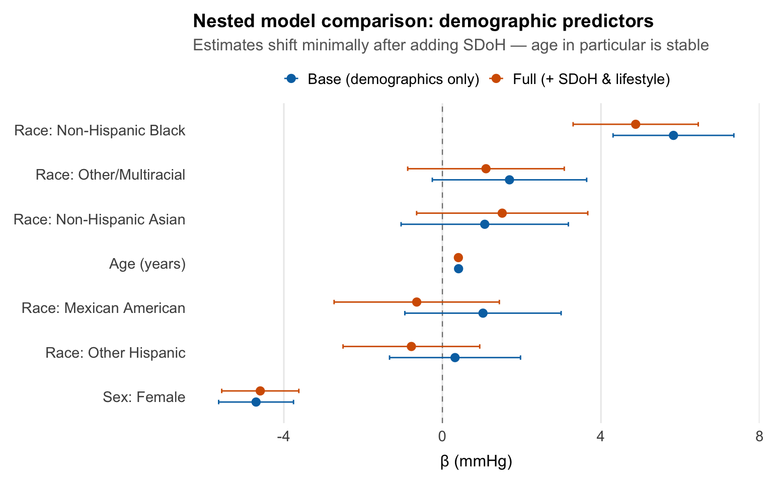
The full SDoH model explained 17.5% of variance in SBP (adjusted R² = 0.171), representing a statistically significant but practically modest improvement over a demographics-only base model (ΔR² = 0.009, F(15, 4853) = 3.59, p < 0.001). Age was the single dominant predictor (β = 0.40 mmHg/year), accounting for much of the variance explained by the base model and showing no attenuation after full adjustment.
Education emerged as the most durable SDoH signal, retaining a monotonic gradient across all levels after mutual adjustment (up to +5.4 mmHg for less than 9th grade vs college graduate). It was the only socioeconomic variable to survive adjustment: poverty-income ratio attenuated to non-significance, its crude association largely absorbed by education. The Non-Hispanic Black-White SBP disparity (+4.9 mmHg adjusted) was not explained by the SDoH variables included in this model; if anything it strengthened slightly after adjustment, pointing to residual factors not captured here.
Several variables with significant crude associations attenuated substantially after adjustment. Physical activity showed no independent association with SBP once other covariates were controlled (β = +0.02, p = 0.8). Waist circumference and diabetes mutually attenuated one another, reflecting shared metabolic variance. Smoking status confounding was confirmed: crude associations (+3.3 and +3.0 mmHg for former and current smokers) were entirely explained by the older age profile of smokers, collapsing to near zero after age adjustment. Food security, sleep hours, and sedentary time showed no significant association in either crude or adjusted analysis.
### Limitations
- **No antihypertensive medication data.** This is the most consequential omission. Treated hypertensives whose SBP remains elevated generate large positive residuals, inflating residual variance and reducing R². Including a medication flag would likely substantially improve model fit and alter several coefficient estimates.
- **Cross-sectional design.** Causal inference is not possible. Associations, particularly the attenuation of physical activity and smoking after adjustment, should be interpreted as descriptive rather than causal.
- **Survey weights not applied.** The model uses unweighted `lm()`, so estimates reflect the analytic sample rather than the US population. NHANES's complex survey design (MEC weights, PSU, strata) is retained in `df_cc` and would need to be incorporated via `survey::svyglm()` for nationally representative inference.
- **Complete case analysis.** `r format(nrow(df) - nrow(df_cc), big.mark = ",")` observations (`r round(100 * (nrow(df) - nrow(df_cc)) / nrow(df), 1)`%) were excluded. While missingness was modest per variable and plausibly random conditional on covariates, some selection bias cannot be ruled out.
- **Self-reported physical activity and sedentary time.** Recall bias and social desirability bias likely introduce measurement error, potentially attenuating associations toward the null.
- **Single SBP measurement.** A single clinic reading is subject to within-person variability and white-coat effects, adding outcome noise.
### Next steps
- Apply survey weights using `survey::svyglm()` for nationally representative estimates.
- Source antihypertensive medication use from NHANES (variable `BPQ050A`) and re-run with a medication flag. This is the highest-priority model extension.
- Explore interaction terms, particularly race × education and race × poverty-income ratio, to assess whether the Non-Hispanic Black SBP disparity varies by socioeconomic position.
- Sensitivity analysis using multiple imputation to assess robustness of complete case findings.
---
## Session Info
```{r}
#| label: session-info
#| collapse: true
#| code-summary: "R session info"
sessionInfo()
```