---
title: "Multiple Linear Regression in R: A Practical Guide"
format:
html:
toc: true
code-fold: true
number-sections: true
execute:
echo: true
warning: false
message: false
editor:
markdown:
wrap: 72
---
# Introduction
This notebook is a practical refresher on multiple linear regression in
R. It is written for someone who already knows the broad idea of
regression, but wants a clear reference for the workflow: how to set up
the data, fit the model, check the assumptions, and interpret the
output without hand-waving.
The example uses systolic blood pressure (SBP) from NHANES 2021–2023.
The aim is not to turn this into a textbook chapter. The aim is to keep
the useful theory close to the code and the modelling decisions, so the
notebook is something you can come back to when you need to get up to
speed quickly.
The main question is straightforward: can we explain variation in SBP
using demographics, social determinants of health, and lifestyle
factors in the same model?
## Where MLR Fits: The GLM Family
Multiple linear regression sits inside the **Generalised Linear Model
(GLM)** family. The main reason to mention that here is practical: it
helps explain why linear, logistic, and Poisson regression feel similar
in R even though they handle different outcome types.
| Model | Outcome type | Distribution | Link function | Coefficient interpretation |
|---|---|---|---|---|
| **Linear regression** | Continuous | Gaussian | Identity | Change in $Y$ per unit change in $X$ |
| **Logistic regression** | Binary (0/1) | Binomial | Logit | Change in log-odds per unit change in $X$ |
| **Poisson regression** | Count | Poisson | Log | Change in log-rate per unit change in $X$ |
In linear regression, the **identity link** means the model works
directly on the outcome scale. Logistic regression uses the **logit
link** because probabilities are bounded between 0 and 1, and Poisson
regression uses the **log link** because counts are non-negative. The
core setup is the same; the outcome distribution and link function are
what change.
::: {.callout-note title="Why does the link function matter?" collapse="true"}
Linear regression assumes the outcome is continuous and unbounded. A
raw probability, however, is bounded between 0 and 1 — so you cannot
directly model it as a linear function of predictors without risking
predicted values outside that range.
The logit link solves this:
$$\log\left(\frac{p}{1-p}\right) = \beta_0 + \beta_1 X_1 + \cdots + \beta_p X_p$$
The left-hand side (log-odds) is unbounded, so a linear predictor on
the right is appropriate. The cost is that coefficients are now in
log-odds units, which are less intuitive to interpret — hence the common
practice of exponentiating them to obtain **odds ratios**.
In linear regression, no such transformation is needed. The identity
link means:
$$E[Y] = \beta_0 + \beta_1 X_1 + \cdots + \beta_p X_p$$
Coefficients are directly interpretable as changes in $Y$.
:::
## The Research Question
This analysis asks: **how much of the variation in systolic blood
pressure can be explained by social and lifestyle factors beyond age,
sex, and race?**
To answer that, we fit two nested models:
- **Base model:** SBP ~ age + sex + race
- **Full model:** SBP ~ age + sex + race + education + poverty ratio +
food security + physical activity + sedentary time + sleep + smoking +
waist circumference + diabetes
---
# Setup and Data Import
## Packages
The package set is small and standard. Nothing here is unusual for an R
regression workflow.
```{r}
#| label: setup
library(here)       # Reproducible file paths
library(tidyverse)  # Data wrangling and visualisation
library(arrow)      # Reading parquet files
library(broom)      # Tidying model output
library(patchwork)  # Combining plots
library(car)        # VIF and diagnostic tests
```
::: {.callout-tip title="Why These Packages?" collapse="true"}
**`here`**
Constructs file paths relative to the project root, so code runs
regardless of where the working directory is set. Essential for
reproducibility. Alternative: `rprojroot`, or simply using absolute
paths (fragile and not portable).
**`tidyverse`**
A collection of packages sharing a common design philosophy. The core
packages used here are:
- `dplyr` — data manipulation (`mutate()`, `filter()`, `select()`)
- `tidyr` — reshaping data (`pivot_longer()`, `drop_na()`)
- `ggplot2` — layered graphics
- `stringr` — string manipulation
- `forcats` — factor handling
Alternative for wrangling: `data.table` (much faster for large
datasets, but with a steeper syntax). For plotting, base R graphics or
`lattice` are alternatives, though `ggplot2` is now the de facto
standard.
**`arrow`**
Reads and writes Apache Parquet files — a columnar storage format that
is compact and fast to read, especially for large datasets. Alternative:
`readr` for CSV, `haven` for Stata/SPSS/SAS files.
**`broom`**
Converts model objects (like `lm`) into tidy data frames. The key
functions are:
- `tidy()` — coefficient table with estimates, SEs, t-statistics,
p-values
- `glance()` — model-level summary (R², F-statistic, AIC, etc.)
- `augment()` — adds fitted values and residuals back to the original
data
Without `broom`, you would extract these manually from `summary(model)`
— which works but is messier.
**`patchwork`**
Combines multiple `ggplot2` objects into a single figure using intuitive
syntax (`p1 | p2` for side-by-side, `p1 / p2` for stacked). Alternative:
`gridExtra::grid.arrange()`.
**`car`**
The *Companion to Applied Regression* package. Used here for:
- `vif()` — variance inflation factors (collinearity diagnostics)
- `ncvTest()` — Breusch-Pagan test for non-constant variance
Alternative for VIF: `performance::check_collinearity()` from the
`performance` package. For the Breusch-Pagan test: `lmtest::bptest()`.
:::
## Data Import and Wrangling
The wrangling pipeline matches the other notebooks in this project. The
main jobs are to clean NHANES sentinel values, derive the physical
activity variable, recode the categorical predictors, and restrict the
analysis to complete cases for the variables used in the model.
```{r}
#| label: import
source(here("R", "plot_theme.R"))

df_raw <- read_parquet(here("data", "processed", "analysis_dataset.parquet"))

df <- df_raw |>
    mutate(
        mod_min_session   = if_else(mod_min_session   %in% c(7777, 9999), NA_real_, mod_min_session),
        vig_min_session   = if_else(vig_min_session   %in% c(7777, 9999), NA_real_, vig_min_session),
        vig_freq          = if_else(vig_freq          %in% c(7777, 9999), NA_real_, vig_freq),
        sedentary_min_day = if_else(sedentary_min_day %in% c(7777, 9999), NA_real_, sedentary_min_day),
        mod_freq_per_week = case_when(
            mod_freq_unit == "D" ~ mod_freq * 7,
            mod_freq_unit == "W" ~ mod_freq,
            mod_freq_unit == "M" ~ mod_freq / 4.3,
            mod_freq_unit == "Y" ~ mod_freq / 52,
            TRUE                 ~ NA_real_
        ),
        vig_freq_per_week = case_when(
            vig_freq_unit == "D" ~ vig_freq * 7,
            vig_freq_unit == "W" ~ vig_freq,
            vig_freq_unit == "M" ~ vig_freq / 4.3,
            vig_freq_unit == "Y" ~ vig_freq / 52,
            TRUE                 ~ NA_real_
        ),
        mod_met       = coalesce(mod_freq_per_week * mod_min_session, 0) * 4,
        vig_met       = coalesce(vig_freq_per_week * vig_min_session, 0) * 8,
        total_met     = mod_met + vig_met,
        log_total_met = log(total_met + 1)
    ) |>
    mutate(
        sex = factor(
            case_when(sex_raw == 1 ~ "Male", sex_raw == 2 ~ "Female"),
            levels = c("Male", "Female")
        ),
        race = factor(
            case_when(
                race_raw == 1 ~ "Mexican American",
                race_raw == 2 ~ "Other Hispanic",
                race_raw == 3 ~ "Non-Hispanic White",
                race_raw == 4 ~ "Non-Hispanic Black",
                race_raw == 6 ~ "Non-Hispanic Asian",
                race_raw == 7 ~ "Other/Multiracial"
            ),
            levels = c(
                "Non-Hispanic White", "Mexican American", "Other Hispanic",
                "Non-Hispanic Black", "Non-Hispanic Asian", "Other/Multiracial"
            )
        ),
        education = factor(
            case_when(
                education_raw == 1         ~ "Less than 9th grade",
                education_raw == 2         ~ "9th-11th grade",
                education_raw == 3         ~ "High school grad / GED",
                education_raw == 4         ~ "Some college / AA degree",
                education_raw == 5         ~ "College graduate or above",
                education_raw %in% c(7, 9) ~ NA_character_
            ),
            levels = c(
                "College graduate or above", "Some college / AA degree",
                "High school grad / GED", "9th-11th grade", "Less than 9th grade"
            )
        ),
        smoking_status = factor(
            case_when(
                ever_smoked == 2                                ~ "Never",
                ever_smoked == 1 & current_smoker == 3         ~ "Former",
                ever_smoked == 1 & current_smoker %in% c(1, 2) ~ "Current",
                TRUE                                            ~ NA_character_
            ),
            levels = c("Never", "Former", "Current")
        ),
        food_security = factor(
            case_when(
                food_security_raw == 1 ~ "Fully food secure",
                food_security_raw == 2 ~ "Marginally food secure",
                food_security_raw == 3 ~ "Low food security",
                food_security_raw == 4 ~ "Very low food security"
            ),
            levels = c(
                "Fully food secure", "Marginally food secure",
                "Low food security", "Very low food security"
            )
        ),
        diabetes_flag = factor(
            case_when(
                diabetes_diagnosis == 1         ~ "Yes",
                diabetes_diagnosis %in% c(2, 3) ~ "No",
                diabetes_diagnosis %in% c(7, 9) ~ NA_character_
            ),
            levels = c("No", "Yes")
        ),
        poverty_ratio = poverty_raw
    )

model_vars <- c(
    "sbp", "log_total_met", "sedentary_min_day", "age", "sex", "race",
    "education", "waist_cm", "poverty_ratio", "sleep_hours", "smoking_status",
    "food_security", "diabetes_flag"
)

df_cc <- df |>
    drop_na(all_of(model_vars)) |>
    select(id, all_of(model_vars), mec_weight, psu, strata)
```
::: {.callout-note title="Why use complete cases?" collapse="true"}
`drop_na(all_of(model_vars))` gives a **complete case analysis (CCA)**:
only participants with non-missing values on every modelling variable
are retained.
That is a pragmatic choice rather than an ideal one. CCA is simplest to
explain and keeps the modelling workflow easy to follow, but it assumes
the excluded records are not introducing serious bias. If missingness
looked more systematic, multiple imputation would be the better next
step.
For this notebook, the tradeoff is acceptable because the complete case
sample ($n =$ `r nrow(df_cc)`) is still large and the goal is to
document the regression workflow clearly.
:::
## Variable Summary
| Variable | Type | Role | Notes |
|---|---|---|---|
| `sbp` | Continuous | Outcome | Systolic blood pressure (mmHg) |
| `age` | Continuous | Predictor | Age in years |
| `sex` | Categorical (2 levels) | Predictor | Reference: Male |
| `race` | Categorical (6 levels) | Predictor | Reference: Non-Hispanic White |
| `education` | Ordinal (5 levels) | Predictor | Reference: College graduate or above |
| `poverty_ratio` | Continuous | Predictor | Income-to-poverty ratio |
| `food_security` | Ordinal (4 levels) | Predictor | Reference: Fully food secure |
| `log_total_met` | Continuous (log-transformed) | Predictor | Physical activity in MET-min/week |
| `sedentary_min_day` | Continuous | Predictor | Sedentary time (min/day) |
| `sleep_hours` | Continuous | Predictor | Self-reported sleep hours/night |
| `smoking_status` | Categorical (3 levels) | Predictor | Reference: Never smoker |
| `waist_cm` | Continuous | Predictor | Waist circumference (cm) |
| `diabetes_flag` | Categorical (2 levels) | Predictor | Reference: No diabetes |
---
# Exploratory Analysis
Before fitting any model, we check the parts of the data that will
drive modelling decisions: the outcome distribution, the shape of the
continuous predictor relationships, and the degree of overlap between
predictors.
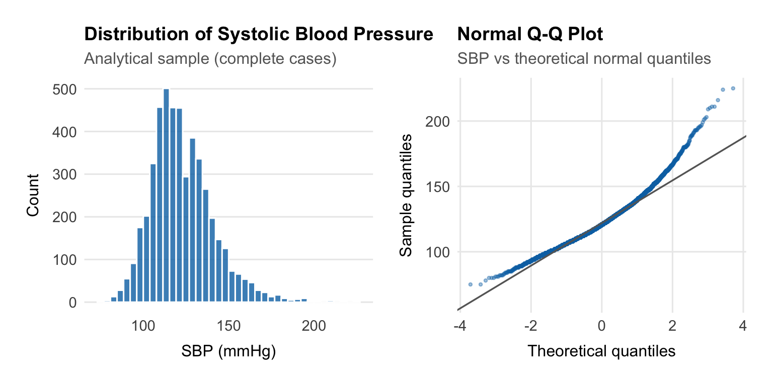
## Outcome Distribution
We begin by examining SBP, the outcome variable.
```{r}
#| label: fig-sbp-dist
#| fig-width: 8
#| fig-height: 4
p_hist <- ggplot(df_cc, aes(x = sbp)) +
    geom_histogram(bins = 40, fill = palette_epi[["blue"]], alpha = 0.8, colour = "white") +
    labs(
        title    = "Distribution of Systolic Blood Pressure",
        subtitle = "Analytical sample (complete cases)",
        x        = "SBP (mmHg)",
        y        = "Count"
    ) +
    theme_epi(grid = "y")

p_qq <- ggplot(df_cc, aes(sample = sbp)) +
    stat_qq(colour = palette_epi[["blue"]], alpha = 0.4, size = 0.8) +
    stat_qq_line(colour = "grey40", linewidth = 0.6) +
    labs(
        title    = "Normal Q-Q Plot",
        subtitle = "SBP vs theoretical normal quantiles",
        x        = "Theoretical quantiles",
        y        = "Sample quantiles"
    ) +
    theme_epi(grid = "both")

p_hist | p_qq
```
Linear regression cares about the **residuals**, not the raw outcome,
but it is still useful to check the outcome first. Here SBP is roughly
symmetric with a mild right tail from higher readings. That is typical
for blood pressure data and does not justify transforming the outcome.
::: {.callout-note title="Does the outcome need to be normally distributed?" collapse="true"}
A common misconception is that MLR requires the outcome variable to be
normally distributed. This is not quite right.
The formal assumption is that the **errors** $\varepsilon_i \sim N(0,
\sigma^2)$ — not the raw outcome. If the model is correctly specified
(the right predictors, the right functional form), the residuals should
be approximately normal even if the raw outcome is mildly skewed.
That said, a severely skewed outcome — for example, a strongly
right-skewed cost variable with a spike at zero — often does produce
non-normal residuals. In such cases, a **log transformation** of the
outcome is common. This changes the interpretation: coefficients then
describe multiplicative rather than additive effects.
For SBP, the distribution is close enough to symmetric that
transformation is not necessary.
:::
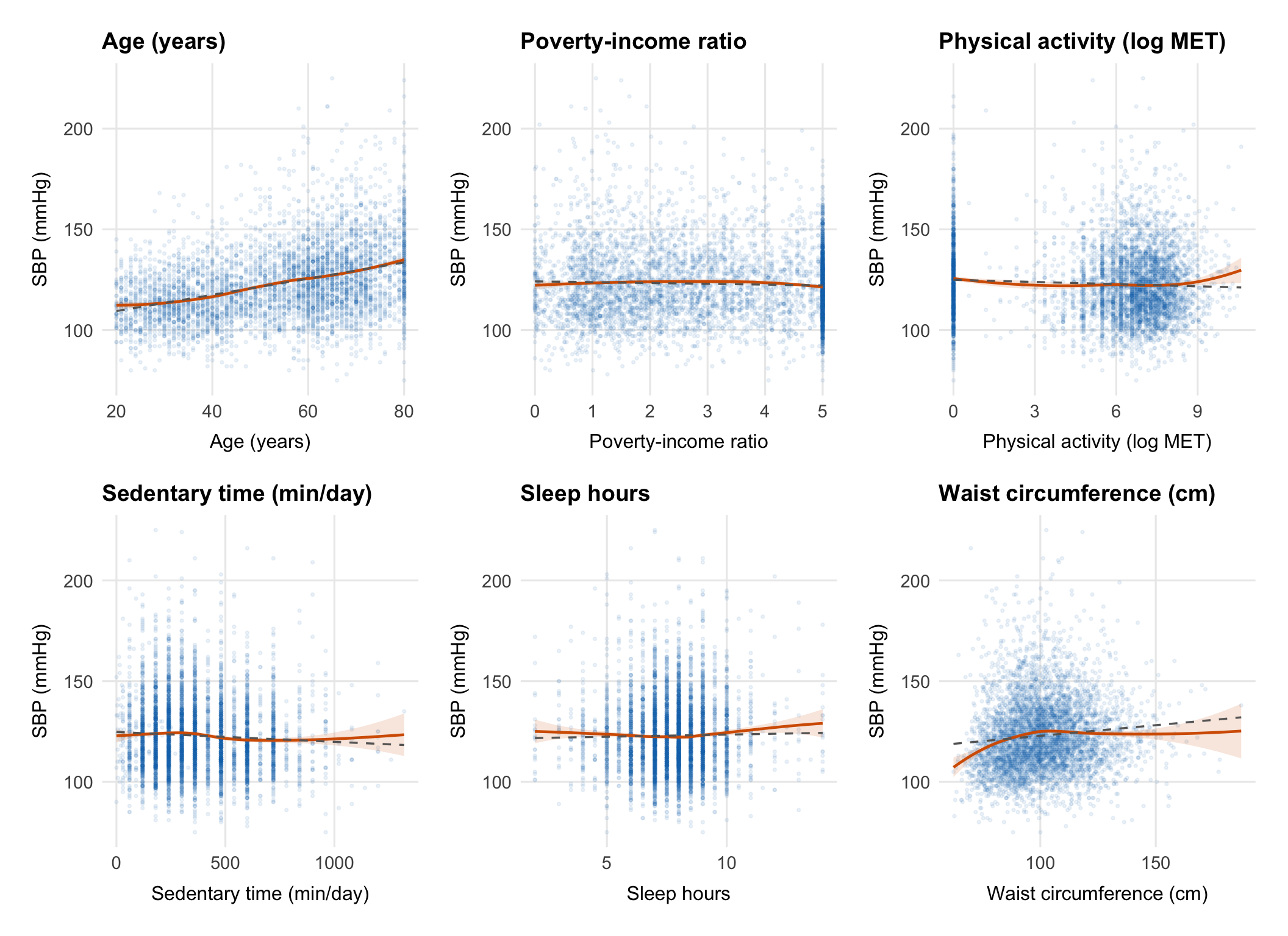
## Linearity Checks
The main question here is whether the continuous predictors look roughly
linear on the SBP scale or whether any of them need a transformation or
more flexible term before we fit the model.
```{r}
#| label: fig-linearity
#| fig-width: 11
#| fig-height: 8
continuous_vars <- c("age", "poverty_ratio", "log_total_met",
                     "sedentary_min_day", "sleep_hours", "waist_cm")

var_labels <- c(
    age             = "Age (years)",
    poverty_ratio   = "Poverty-income ratio",
    log_total_met   = "Physical activity (log MET)",
    sedentary_min_day = "Sedentary time (min/day)",
    sleep_hours     = "Sleep hours",
    waist_cm        = "Waist circumference (cm)"
)

plots <- map(continuous_vars, function(var) {
    ggplot(df_cc, aes(x = .data[[var]], y = sbp)) +
        geom_point(alpha = 0.08, size = 0.6, colour = palette_epi[["blue"]]) +
        geom_smooth(method = "loess", se = TRUE, colour = palette_epi[["vermillion"]],
                    linewidth = 0.8, fill = palette_epi[["vermillion"]], alpha = 0.15) +
        geom_smooth(method = "lm", se = FALSE, colour = "grey40",
                    linewidth = 0.6, linetype = "dashed") +
        labs(
            title = var_labels[var],
            x     = var_labels[var],
            y     = "SBP (mmHg)"
        ) +
        theme_epi(grid = "both")
})

wrap_plots(plots, ncol = 3)
```
Each panel compares a LOESS smooth (red) with a straight-line fit
(dashed grey). If they track closely, a linear term is probably fine.
If they diverge, that predictor may need a transformation or spline.
::: {.callout-note title="What is LOESS and why use it here?" collapse="true"}
**LOESS** (Locally Estimated Scatterplot Smoothing) is a
non-parametric smoother that fits a local regression at each point in
the data using a weighted neighbourhood of observations. It makes no
assumption about the global shape of the relationship — it simply lets
the data speak.
This makes it ideal for checking whether the assumption of linearity is
reasonable. If the LOESS curve is approximately straight, a linear term
is defensible. If it curves meaningfully, you have options:
- **Log-transform the predictor** (useful for right-skewed predictors
with a decelerating relationship)
- **Add a polynomial term** (e.g., $X + X^2$ for a quadratic
relationship)
- **Use a spline** (e.g., `ns(X, df = 3)` for a flexible smooth curve
that doesn't assume any specific shape)
The physical activity predictor (`total_met`) is already
log-transformed here because the raw MET distribution is extremely
right-skewed and the relationship with SBP is approximately
log-linear.
:::
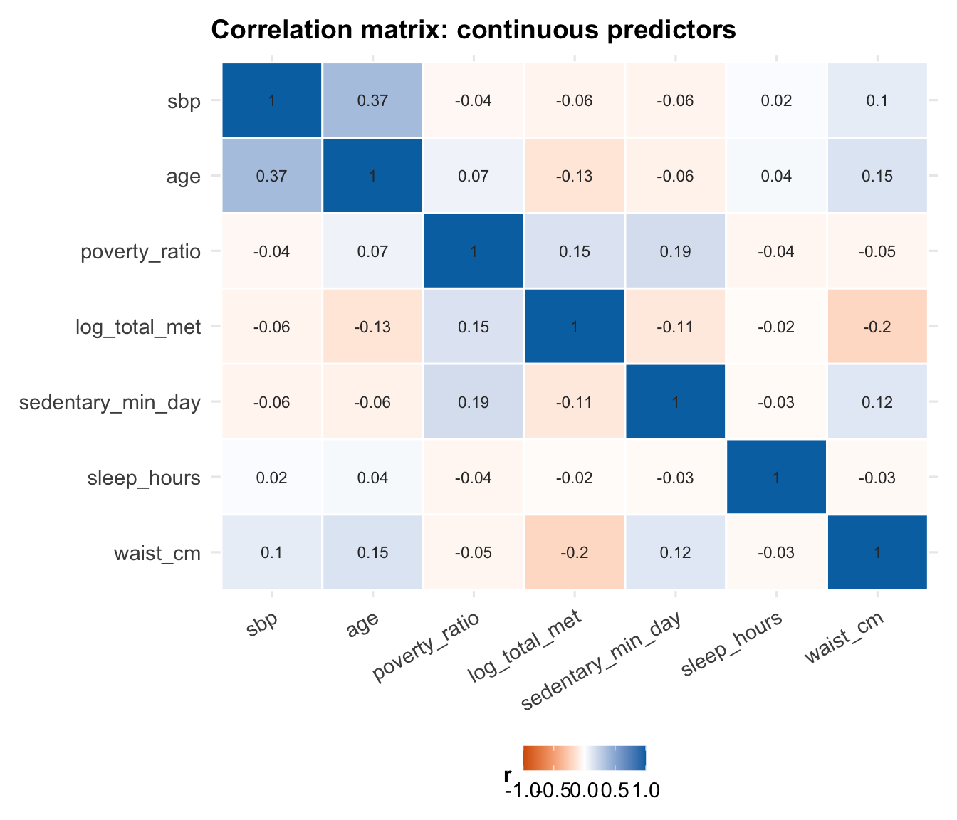
## Collinearity
Before fitting the model, it is also worth checking whether any
continuous predictors are so correlated that they are likely to cause
interpretation or stability problems later.
```{r}
#| label: fig-correlation
#| fig-width: 7
#| fig-height: 6
cor_data <- df_cc |>
    select(sbp, age, poverty_ratio, log_total_met,
           sedentary_min_day, sleep_hours, waist_cm) |>
    cor(use = "complete.obs")

cor_data |>
    as.data.frame() |>
    rownames_to_column("var1") |>
    pivot_longer(-var1, names_to = "var2", values_to = "r") |>
    mutate(
        var1 = factor(var1, levels = colnames(cor_data)),
        var2 = factor(var2, levels = rev(colnames(cor_data)))
    ) |>
    ggplot(aes(x = var1, y = var2, fill = r)) +
    geom_tile(colour = "white", linewidth = 0.5) +
    geom_text(aes(label = round(r, 2)), size = 3, colour = "grey20") +
    scale_fill_gradient2(
        low      = palette_epi[["vermillion"]],
        mid      = "white",
        high     = palette_epi[["blue"]],
        midpoint = 0,
        limits   = c(-1, 1)
    ) +
    labs(
        title = "Correlation matrix: continuous predictors",
        x     = NULL,
        y     = NULL,
        fill  = "r"
    ) +
    theme_epi() +
    theme(axis.text.x = element_text(angle = 30, hjust = 1))
```
::: {.callout-note title="What is collinearity and why does it matter?" collapse="true"}
**Collinearity** (or multicollinearity) occurs when two or more
predictors in a regression model are highly correlated with each other.
This matters because MLR estimates the effect of each predictor
**holding all others constant**. When two predictors move together,
there is little independent variation in each to work with. The model
struggles to distinguish their separate effects, and the result is:
- **Inflated standard errors** — the confidence intervals on
coefficients widen substantially
- **Unstable estimates** — small changes in the data can cause large
swings in the estimated coefficients
- **Difficult interpretation** — the coefficient for $X_1$ represents
its effect "holding $X_2$ constant", but if $X_1$ and $X_2$ almost
always move together in the real world, this conditional effect is
rarely observed
Collinearity does **not** bias coefficient estimates — it just makes
them imprecise. It also does not affect the model's predictive
performance if future data come from the same distribution.
We quantify collinearity after fitting the model using **Variance
Inflation Factors (VIFs)** — see the diagnostics section.
:::
---
# The Multiple Linear Regression Model
This section keeps the theory that is most useful when reading model
output. The goal is not to reproduce a full regression lecture, but to
keep the key ideas close to the analysis.
## The Model Equation
In multiple linear regression, we model the expected value of a
continuous outcome $Y$ as a linear function of $p$ predictors:
$$Y_i = \beta_0 + \beta_1 X_{i1} + \beta_2 X_{i2} + \cdots + \beta_p X_{ip} + \varepsilon_i$$
where:
- $Y_i$ is the observed outcome for subject $i$ (SBP in mmHg)
- $\beta_0$ is the **intercept** — the expected value of $Y$ when all
predictors equal zero
- $\beta_j$ is the **partial regression coefficient** for predictor $j$
— the expected change in $Y$ for a one-unit increase in $X_j$, **holding
all other predictors constant**
- $\varepsilon_i$ is the **error term** — the part of $Y_i$ not
explained by the predictors
The errors are assumed to be independent and identically distributed:
$\varepsilon_i \overset{iid}{\sim} N(0, \sigma^2)$.
## Matrix Form
For $n$ observations and $p$ predictors, the model is written compactly
in matrix form:
$$\mathbf{Y} = \mathbf{X}\boldsymbol{\beta} + \boldsymbol{\varepsilon}$$
where:
$$\mathbf{Y} = \begin{pmatrix} Y_1 \\ Y_2 \\ \vdots \\ Y_n \end{pmatrix}, \quad
\mathbf{X} = \begin{pmatrix} 1 & X_{11} & \cdots & X_{1p} \\ 1 & X_{21} & \cdots & X_{2p} \\ \vdots & \vdots & \ddots & \vdots \\ 1 & X_{n1} & \cdots & X_{np} \end{pmatrix}, \quad
\boldsymbol{\beta} = \begin{pmatrix} \beta_0 \\ \beta_1 \\ \vdots \\ \beta_p \end{pmatrix}, \quad
\boldsymbol{\varepsilon} = \begin{pmatrix} \varepsilon_1 \\ \varepsilon_2 \\ \vdots \\ \varepsilon_n \end{pmatrix}$$
$\mathbf{X}$ is the **design matrix** — an $n \times (p+1)$ matrix with
a column of ones (for the intercept) and one column per predictor.
::: {.callout-note title="Ordinary Least Squares: deriving the coefficient estimates" collapse="true"}
The goal of OLS is to find the coefficient vector $\hat{\boldsymbol{\beta}}$ that
minimises the **residual sum of squares**:
$$SS_{res} = \sum_{i=1}^n (Y_i - \hat{Y}_i)^2 = (\mathbf{Y} - \mathbf{X}\boldsymbol{\beta})^\top(\mathbf{Y} - \mathbf{X}\boldsymbol{\beta})$$
To minimise, we differentiate with respect to $\boldsymbol{\beta}$ and
set to zero:
$$\frac{\partial SS_{res}}{\partial \boldsymbol{\beta}} = -2\mathbf{X}^\top(\mathbf{Y} - \mathbf{X}\boldsymbol{\beta}) = \mathbf{0}$$
Rearranging gives the **normal equations**:
$$\mathbf{X}^\top\mathbf{X}\hat{\boldsymbol{\beta}} = \mathbf{X}^\top\mathbf{Y}$$
Provided $\mathbf{X}^\top\mathbf{X}$ is invertible (i.e., the predictors
are not perfectly collinear), the unique solution is:
$$\hat{\boldsymbol{\beta}} = (\mathbf{X}^\top\mathbf{X})^{-1}\mathbf{X}^\top\mathbf{Y}$$
This is the **OLS estimator**. It is the Best Linear Unbiased Estimator
(BLUE) under the Gauss-Markov assumptions — it has the smallest
variance of any linear unbiased estimator.
The **fitted values** are:
$$\hat{\mathbf{Y}} = \mathbf{X}\hat{\boldsymbol{\beta}} = \mathbf{X}(\mathbf{X}^\top\mathbf{X})^{-1}\mathbf{X}^\top\mathbf{Y} = \mathbf{H}\mathbf{Y}$$
where $\mathbf{H} = \mathbf{X}(\mathbf{X}^\top\mathbf{X})^{-1}\mathbf{X}^\top$ is
called the **hat matrix** (it puts the "hat" on $\mathbf{Y}$). The
diagonal elements $h_{ii}$ measure the **leverage** of each observation
— how much influence it has on its own fitted value. We return to this
in the diagnostics section.
The **residuals** are:
$$\mathbf{e} = \mathbf{Y} - \hat{\mathbf{Y}} = (\mathbf{I} - \mathbf{H})\mathbf{Y}$$
The variance of the coefficient estimates is:
$$\text{Var}(\hat{\boldsymbol{\beta}}) = \sigma^2 (\mathbf{X}^\top\mathbf{X})^{-1}$$
Since $\sigma^2$ is unknown, we estimate it with the **mean squared
error**:
$$\hat{\sigma}^2 = MSE = \frac{SS_{res}}{n - p - 1}$$
where $n - p - 1$ is the degrees of freedom (sample size minus the
number of estimated parameters). The square root $\hat{\sigma} =
\sqrt{MSE}$ is the **residual standard error** reported by R's
`summary()`.
:::
## Model Assumptions
The standard assumptions are worth keeping in view because almost all of
the diagnostics later in the notebook are checking one of them.
### Linearity
The relationship between each predictor and the outcome is linear in
the parameters. This is checked graphically (scatter plots with LOESS
smoothers, residuals vs fitted plot).
### Independence
Observations are independent of each other. This is violated by
clustered data (e.g., patients within hospitals), repeated measures, or
time series. Violations require mixed effects models, GEE, or time
series methods.
::: {.callout-note title="Survey data and independence" collapse="true"}
NHANES uses a **complex survey design** — a stratified, multistage
probability sample. Participants within the same primary sampling unit
(PSU) may be more similar to each other than to participants from
different PSUs, violating the independence assumption.
A fully correct analysis would use survey-weighted regression via
`survey::svyglm()`, incorporating the sampling weights (`mec_weight`),
PSU (`psu`), and strata (`strata`) variables. This adjusts both
coefficient estimates and standard errors.
For simplicity and pedagogical clarity, this notebook uses unweighted
OLS. The regression notebook in this project uses the same approach.
The substantive findings are unlikely to change dramatically, but
standard errors may be slightly underestimated.
:::
### Normality of Residuals
The residuals $\varepsilon_i$ are normally distributed. This assumption
is needed for valid inference (t-tests and F-tests on coefficients).
With large samples, the central limit theorem means that
non-normality has little practical impact on p-values — but it can
affect prediction intervals.
### Equal Variance (Homoscedasticity)
The variance of the residuals is constant across all fitted values:
$\text{Var}(\varepsilon_i) = \sigma^2$ for all $i$. When this fails
(**heteroscedasticity**), OLS estimates remain unbiased but standard
errors are incorrect — leading to invalid inference.
::: {.callout-note title="What to do when assumptions are violated" collapse="true"}
| Violated assumption | Consequence | Remedies |
|---|---|---|
| **Non-linearity** | Biased coefficients, poor fit | Transform predictor, add polynomial term, use spline |
| **Non-independence** | Underestimated SEs, anti-conservative p-values | Mixed effects model, GEE, cluster-robust SEs |
| **Non-normality** | Invalid inference in small samples | Log-transform outcome, use robust regression |
| **Heteroscedasticity** | Biased SEs, invalid inference | Heteroscedasticity-robust SEs (`vcovHC`), weighted least squares, transform outcome |
In large samples ($n > 500$), mild violations of normality and
homoscedasticity rarely have a meaningful impact on inference. The
independence assumption is the one that tends to matter most regardless
of sample size.
:::
## Categorical Predictors and Dummy Coding
Categorical variables cannot enter a regression model directly — they
must be represented as a set of **dummy (indicator) variables**.
For a categorical variable with $k$ levels, R creates $k - 1$ dummy
variables. Each dummy compares one level to the **reference group**
(the omitted category). For example, with race coded as:
| Variable | Meaning |
|---|---|
| `raceMexican American` | 1 if Mexican American, 0 otherwise |
| `raceOther Hispanic` | 1 if Other Hispanic, 0 otherwise |
| `raceNon-Hispanic Black` | 1 if Non-Hispanic Black, 0 otherwise |
| `raceNon-Hispanic Asian` | 1 if Non-Hispanic Asian, 0 otherwise |
| `raceOther/Multiracial` | 1 if Other/Multiracial, 0 otherwise |
The **reference group** is Non-Hispanic White — the level not
represented by any dummy. Its effect is absorbed into the intercept.
Each coefficient for race represents the **difference in mean SBP
between that group and Non-Hispanic White**, holding all other
predictors constant.
::: {.callout-note title="Why $k - 1$ dummies and not $k$?" collapse="true"}
If we created a dummy variable for every level of a categorical
variable, the columns of the design matrix $\mathbf{X}$ would be
perfectly collinear — they would sum to 1 (the intercept column) for
every row. This is called **perfect multicollinearity**, and it makes
$\mathbf{X}^\top\mathbf{X}$ singular (non-invertible), so the OLS
estimator $(\mathbf{X}^\top\mathbf{X})^{-1}$ does not exist.
The fix is to drop one level — the reference group — so that the
remaining dummies are not a linear combination of each other or of the
intercept.
The choice of reference group does not affect model fit, predicted
values, or the overall F-test. It only affects the interpretation of
the individual dummy coefficients — each is now relative to the chosen
reference.
In R, the reference level is set by factor ordering. The first level
of the factor becomes the reference. We can change this with
`relevel(factor_var, ref = "new_reference")`.
:::
---
# Model Building
## Base Model
We start with a simple demographic model. That gives us a baseline
before adding the social and lifestyle predictors.
```{r}
#| label: model-base
model_base <- lm(sbp ~ age + sex + race, data = df_cc)
summary(model_base)
```
::: {.callout-note title="Reading the R summary output" collapse="true"}
The `summary()` output for an `lm` object contains several key
components:
**Residuals**
A five-number summary of the raw residuals. If the model fits well and
residuals are symmetric, the min/max should be roughly equal in
magnitude, and the median should be close to zero.
**Coefficients table**
| Column | Meaning |
|---|---|
| `Estimate` | The estimated coefficient $\hat{\beta}_j$ |
| `Std. Error` | The standard error $SE(\hat{\beta}_j) = \sqrt{\hat{\sigma}^2 [(\mathbf{X}^\top\mathbf{X})^{-1}]_{jj}}$ |
| `t value` | The test statistic $t = \hat{\beta}_j / SE(\hat{\beta}_j)$, used to test $H_0: \beta_j = 0$ |
| `Pr(>|t|)` | Two-tailed p-value from the t-distribution with $n - p - 1$ degrees of freedom |
**Residual standard error**
$\hat{\sigma} = \sqrt{MSE}$ — the estimated standard deviation of the
residuals. Smaller values indicate better fit. The degrees of freedom
shown ($n - p - 1$) confirm how many parameters were estimated.
**R-squared**
The proportion of variance in $Y$ explained by the model (see Section 6).
**F-statistic**
Tests whether the model as a whole explains significantly more variance
than an intercept-only model. The associated p-value tests $H_0: \beta_1
= \beta_2 = \cdots = \beta_p = 0$.
:::
## Full Model
The full model adds the social and lifestyle variables used throughout
the project.
```{r}
#| label: model-full
model_full <- lm(
    sbp ~ age + sex + race +
          log_total_met + sedentary_min_day +
          waist_cm + education + poverty_ratio +
          sleep_hours + smoking_status +
          food_security + diabetes_flag,
    data = df_cc
)
summary(model_full)
```
::: {.callout-note title="Why build models incrementally?" collapse="true"}
Fitting the base model before the full model is not just convention —
it serves several purposes:
**1. Establishes a baseline for comparison.**
Without a reference point, we cannot quantify what the additional
predictors add. The nested model comparison (Section 6) is only
possible because we have both models.
**2. Reveals confounding.**
If a coefficient changes substantially when we add predictors, it
suggests the original association was confounded. For example, if the
age coefficient changed after adding smoking status, it would suggest
the two are correlated and that the crude age effect was partly
reflecting the older age profile of smokers (or vice versa).
**3. Supports a clear narrative.**
"Demographics alone explain X%; adding social factors explains Y%"
is a more compelling and interpretable finding than presenting a single
full model in isolation.
**4. Parsimony.**
Not all variables need to be in the final model. A model with fewer
predictors that fits nearly as well is preferable — it is more
interpretable, less prone to overfitting, and more robust to new data.
:::
---
# Nested Model Comparison
## Sums of Squares
To compare the base and full models, we need a compact way to describe
fit and improvement.
$$SS_{tot} = SS_{reg} + SS_{res}$$
$$\underbrace{\sum_{i=1}^n (Y_i - \bar{Y})^2}_{SS_{tot}} = \underbrace{\sum_{i=1}^n (\hat{Y}_i - \bar{Y})^2}_{SS_{reg}} + \underbrace{\sum_{i=1}^n (Y_i - \hat{Y}_i)^2}_{SS_{res}}$$
where:
- $SS_{tot}$ (total sum of squares) — total variability in $Y$ around
its mean
- $SS_{reg}$ (regression sum of squares) — variability explained by the
model
- $SS_{res}$ (residual sum of squares) — variability not explained by
the model (unexplained error)
## R-Squared
**R-squared** ($R^2$) is the proportion of total variance explained by
the model:
$$R^2 = \frac{SS_{reg}}{SS_{tot}} = 1 - \frac{SS_{res}}{SS_{tot}}$$
$R^2 \in [0, 1]$, where 0 means the model explains nothing and 1 means
perfect fit.
::: {.callout-warning title="A critical limitation of R²" collapse="true"}
$R^2$ **never decreases** when you add a predictor to the model, even
if that predictor is pure noise. This is because any additional
predictor will absorb at least some residual variance by chance.
This makes $R^2$ a poor criterion for model comparison when models
differ in the number of predictors.
**Adjusted R²** penalises for the number of predictors:
$$\bar{R}^2 = 1 - \frac{SS_{res}/(n - p - 1)}{SS_{tot}/(n - 1)} = 1 - (1 - R^2)\frac{n-1}{n-p-1}$$
Adjusted $R^2$ **can decrease** when a predictor adds less explanatory
power than would be expected by chance. It is a better measure of
model quality when comparing models with different numbers of
predictors.
Neither $R^2$ nor adjusted $R^2$ tells you whether the model is
correctly specified — a high $R^2$ with systematically curved
residuals still indicates a bad model.
:::
## The F-Test for Nested Model Comparison
The formal comparison is an **extra sum of squares F-test**. In plain
terms, it asks whether the extra predictors in the full model reduce the
remaining error enough to matter beyond chance.
Let the **reduced model** (base) have $p_R$ predictors and residual sum
of squares $SS_{res,R}$, and the **full model** have $p_F > p_R$
predictors and $SS_{res,F}$. The number of additional parameters is $q
= p_F - p_R$.
The F-statistic is:
$$F = \frac{(SS_{res,R} - SS_{res,F})\, /\, q}{SS_{res,F}\, /\, (n - p_F - 1)}$$
Under $H_0$ (the additional predictors have no effect), this statistic
follows an $F(q,\, n - p_F - 1)$ distribution. A large F (and small
p-value) indicates the additional predictors jointly explain a
statistically significant amount of additional variance.
::: {.callout-note title="Intuition behind the F-statistic" collapse="true"}
The numerator of the F-statistic measures how much the residual sum of
squares **decreases** when we add the extra $q$ predictors, divided by
$q$ (to get an average improvement per predictor).
The denominator is the residual mean squared error of the full model —
a measure of the noise floor.
If the ratio is large, the additional predictors are reducing
unexplained variance meaningfully relative to the background noise. If
the ratio is close to 1, the gain in explained variance is no more than
we would expect by chance.
The $F(q, n - p_F - 1)$ distribution provides the reference: if $H_0$
is true, what values of $F$ are plausible? A p-value is then the
probability of observing an $F$ as large as or larger than the observed
value under $H_0$.
:::
```{r}
#| label: model-comparison
anova(model_base, model_full)
```
::: {.callout-note title="How to report a nested model comparison" collapse="true"}
A complete report of the model comparison should include:
1. The R² of both models
2. The change in R² ($\Delta R^2$)
3. The F-statistic with its degrees of freedom
4. The associated p-value
**Example reporting:**
> The full model (including social determinants and lifestyle variables)
> explained 17.45% of the variance in SBP ($R^2 = 0.175$), compared to
> 16.54% for the base demographic model ($R^2 = 0.165$). The additional
> predictors jointly explained a statistically significant increment of
> variance ($\Delta R^2 = 0.009$, $F(15, 4853) = 3.59$, $p < 0.001$).
Note the distinction between **statistical significance** and **practical
significance**. A $\Delta R^2$ of 0.009 is real — the F-test confirms
it is unlikely to be due to chance — but it is small. In a clinical
context, a model that explains 17.45% of SBP variance rather than
16.54% does not represent a meaningful improvement in prediction.
**What counts as a meaningful $R^2$?** There is no universal threshold.
In social science and epidemiology, models explaining 10–30% of variance
are common for complex behaviours and outcomes with many unmeasured
drivers. In controlled laboratory settings, $R^2 > 0.90$ is routine. The
appropriate benchmark depends on the discipline and the nature of the
outcome.
:::
```{r}
#| label: r2-table
tibble(
    Model     = c("Base (age + sex + race)", "Full (+ SDoH & lifestyle)"),
    R2        = c(summary(model_base)$r.squared, summary(model_full)$r.squared),
    Adj_R2    = c(summary(model_base)$adj.r.squared, summary(model_full)$adj.r.squared),
    Sigma     = c(summary(model_base)$sigma, summary(model_full)$sigma)
) |>
    mutate(across(c(R2, Adj_R2), ~ round(., 4)),
           Sigma = round(Sigma, 3)) |>
    knitr::kable(
        col.names = c("Model", "R²", "Adjusted R²", "Residual SE"),
        caption   = "Model comparison: variance explained"
    )
```
---
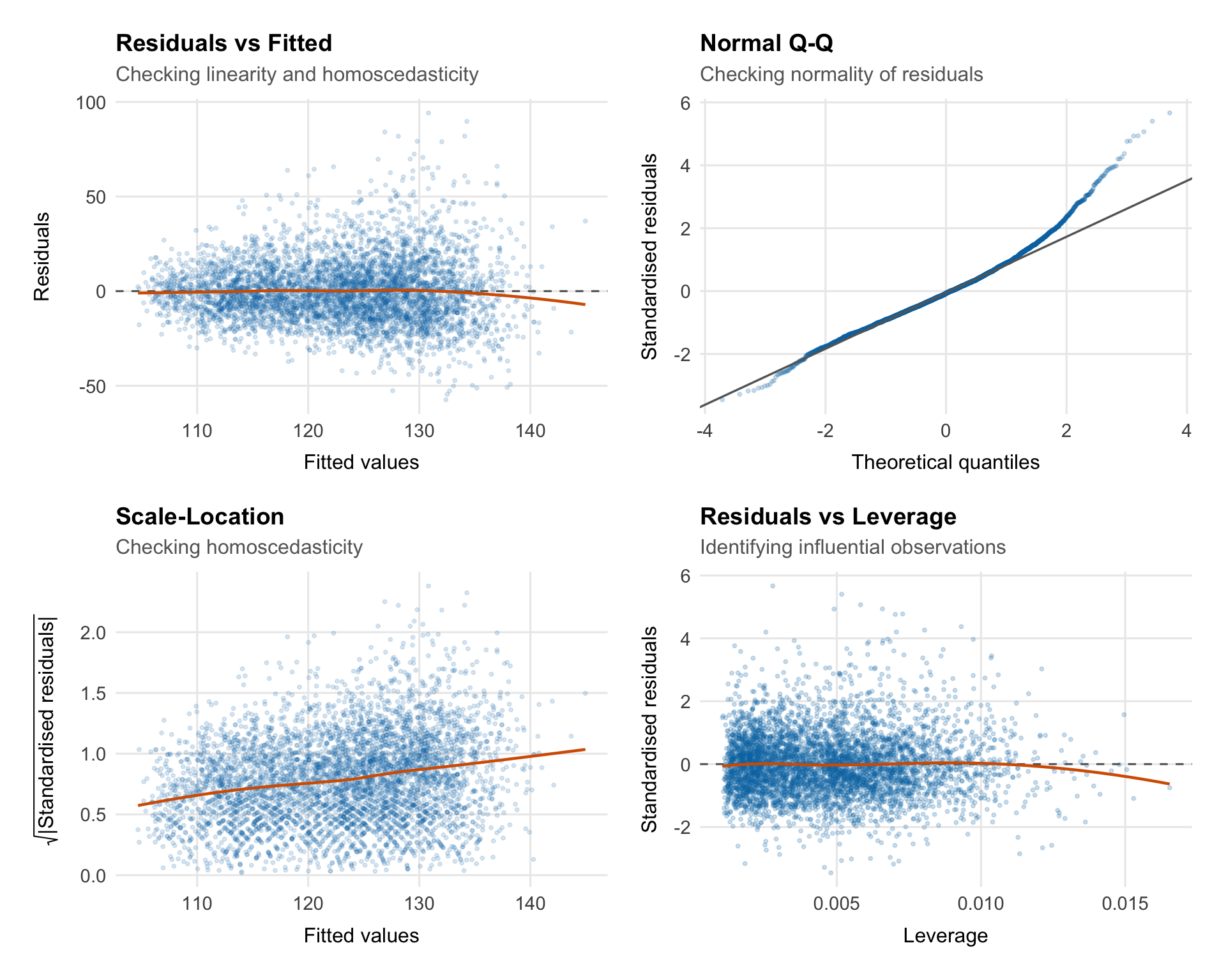
# Model Diagnostics
Fitting the model is only the start. Before interpreting coefficients or
p-values, we need to see whether the residuals look consistent with the
assumptions of ordinary least squares.
## What Are Residuals?
For each observation $i$, the **raw residual** is the difference
between the observed and fitted value:
$$e_i = Y_i - \hat{Y}_i$$
Residuals are the part of SBP the model leaves unexplained. If the model
is behaving reasonably:
- Residuals should be centred around zero
- Residuals should have constant variance across fitted values
- Residuals should be approximately normally distributed
- Residuals should be independent (no patterns over time or across groups)
We use several diagnostic plots to check these properties.
::: {.callout-note title="Raw vs standardised vs studentised residuals" collapse="true"}
**Raw residuals** $e_i = Y_i - \hat{Y}_i$ are on the scale of the
outcome and have unequal variances — observations with high leverage
tend to have smaller residuals because the model is pulled toward them.
**Standardised residuals** divide by an estimate of the residual
standard deviation:
$$r_i = \frac{e_i}{\hat{\sigma}\sqrt{1 - h_{ii}}}$$
where $h_{ii}$ is the leverage of observation $i$ (the $i$-th diagonal
element of the hat matrix $\mathbf{H}$). Standardised residuals should
be approximately $N(0, 1)$, so values beyond $\pm 2$ or $\pm 3$ suggest
potential outliers.
**Studentised (externally studentised) residuals** go one step further
— they refit the model without observation $i$ and use that model's
$\hat{\sigma}_{-i}$ to standardise:
$$t_i = \frac{e_i}{\hat{\sigma}_{-i}\sqrt{1 - h_{ii}}}$$
These follow a $t_{n-p-2}$ distribution and are more sensitive to
outliers. R's `rstudent()` function returns these.
:::
## Diagnostic Plots
```{r}
#| label: fig-diagnostics
#| fig-width: 10
#| fig-height: 8
aug <- augment(model_full)

p1 <- ggplot(aug, aes(x = .fitted, y = .resid)) +
    geom_point(alpha = 0.15, size = 0.7, colour = palette_epi[["blue"]]) +
    geom_hline(yintercept = 0, linetype = "dashed", colour = "grey40") +
    geom_smooth(method = "loess", se = FALSE, colour = palette_epi[["vermillion"]],
                linewidth = 0.8) +
    labs(title    = "Residuals vs Fitted",
         subtitle = "Checking linearity and homoscedasticity",
         x        = "Fitted values",
         y        = "Residuals") +
    theme_epi(grid = "both")

p2 <- ggplot(aug, aes(sample = .std.resid)) +
    stat_qq(alpha = 0.2, size = 0.7, colour = palette_epi[["blue"]]) +
    stat_qq_line(colour = "grey40", linewidth = 0.6) +
    labs(title    = "Normal Q-Q",
         subtitle = "Checking normality of residuals",
         x        = "Theoretical quantiles",
         y        = "Standardised residuals") +
    theme_epi(grid = "both")

p3 <- ggplot(aug, aes(x = .fitted, y = sqrt(abs(.std.resid)))) +
    geom_point(alpha = 0.15, size = 0.7, colour = palette_epi[["blue"]]) +
    geom_smooth(method = "loess", se = FALSE, colour = palette_epi[["vermillion"]],
                linewidth = 0.8) +
    labs(title    = "Scale-Location",
         subtitle = "Checking homoscedasticity",
         x        = "Fitted values",
         y        = expression(sqrt("|Standardised residuals|"))) +
    theme_epi(grid = "both")

p4 <- ggplot(aug, aes(x = .hat, y = .std.resid)) +
    geom_point(alpha = 0.2, size = 0.7, colour = palette_epi[["blue"]]) +
    geom_hline(yintercept = 0, linetype = "dashed", colour = "grey40") +
    geom_smooth(method = "loess", se = FALSE, colour = palette_epi[["vermillion"]],
                linewidth = 0.8) +
    labs(title    = "Residuals vs Leverage",
         subtitle = "Identifying influential observations",
         x        = "Leverage",
         y        = "Standardised residuals") +
    theme_epi(grid = "both")

(p1 | p2) / (p3 | p4)
```
### Residuals vs Fitted
::: {.callout-note title="What this plot checks — and what to look for" collapse="true"}
**What it checks:** Linearity and homoscedasticity simultaneously.
**The x-axis** shows the fitted values $\hat{Y}_i$ — the model's
predictions. **The y-axis** shows the raw residuals $e_i = Y_i -
\hat{Y}_i$.
**What we want to see:**
- Points scattered randomly around zero with no systematic pattern
- Roughly equal spread across the range of fitted values
- The LOESS smoother (red line) should be approximately flat at zero
**What would concern us:**
- A **curve** in the LOESS smoother suggests non-linearity — some
predictor(s) have a non-linear effect that the model is not capturing
- A **funnel shape** (spread increasing with fitted values) indicates
heteroscedasticity — the variance of errors is not constant
- A **horizontal band** that widens or narrows suggests the same
**What to do if this fails:**
- Non-linearity: add polynomial terms, splines, or transform the
predictor(s)
- Heteroscedasticity: use heteroscedasticity-robust standard errors
(`sandwich::vcovHC()`), weighted least squares, or transform the
outcome
:::
### Normal Q-Q Plot
::: {.callout-note title="What this plot checks — and what to look for" collapse="true"}
**What it checks:** Normality of residuals.
A Q-Q plot compares the **empirical quantiles** of the standardised
residuals against the **theoretical quantiles** of a standard normal
distribution. If the residuals are normally distributed, the points
should fall on the diagonal reference line.
**What we want to see:**
- Points tracking closely along the diagonal line
**What would concern us:**
- **Heavy tails** (points curving away from the line at both ends)
indicate a distribution with more extreme values than the normal
— the model is producing more large residuals than expected
- **Light tails** (points flatter than the line at the ends) indicate
fewer extremes than the normal
- **Systematic curvature** (S-shaped pattern) indicates skewness in the
residuals
**What to do if this fails:**
In large samples ($n > 500$), moderate departures from normality have
little effect on inference — the central limit theorem ensures that
coefficient estimates are approximately normally distributed regardless.
For smaller samples or severe non-normality, consider transforming the
outcome or using bootstrap confidence intervals.
:::
### Scale-Location
::: {.callout-note title="What this plot checks — and what to look for" collapse="true"}
**What it checks:** Homoscedasticity (equal variance).
Also called the **spread-location plot**, this plots $\sqrt{|r_i|}$
(the square root of the absolute standardised residuals) against fitted
values. The square root transformation stabilises the scale and makes
trends in spread easier to detect.
**What we want to see:**
- A roughly horizontal LOESS smoother
- Points scattered evenly across the range of fitted values
**What would concern us:**
- An **upward slope** indicates increasing variance with fitted values
(the most common form of heteroscedasticity)
- A **downward slope** indicates decreasing variance
- Any systematic trend is a problem
**A formal test:** The Breusch-Pagan test (`car::ncvTest()`) provides a
p-value for the null hypothesis of constant variance.
:::
```{r}
#| label: breusch-pagan
car::ncvTest(model_full)
```
### Residuals vs Leverage
::: {.callout-note title="Leverage, influence, and Cook's Distance" collapse="true"}
**Leverage** measures how unusual an observation's predictor values
are — how far the observation is from the centre of the predictor
space. The leverage of observation $i$ is the $i$-th diagonal element
of the hat matrix:
$$h_{ii} = [\mathbf{H}]_{ii} = [\mathbf{X}(\mathbf{X}^\top\mathbf{X})^{-1}\mathbf{X}^\top]_{ii}$$
$h_{ii}$ ranges from $1/n$ to 1. High leverage observations have
unusual predictor values. They may or may not be **influential** —
that depends on whether their residual is also large.
**Influence** combines leverage and residual size. The most widely used
measure is **Cook's Distance**:
$$D_i = \frac{e_i^2}{(p+1)\, MSE} \cdot \frac{h_{ii}}{(1 - h_{ii})^2}$$
Cook's $D_i$ measures how much the entire vector of fitted values
changes if observation $i$ is removed from the dataset. It combines the
size of the residual (numerator) with the leverage (denominator).
Common rules of thumb:
- $D_i > 1$: potentially influential
- $D_i > 4/n$: a more conservative threshold often used in practice
**The Residuals vs Leverage plot** helps identify observations that are
both high leverage and high residual — the most dangerous combination.
Cook's distance contours are sometimes overlaid (dashed lines) to mark
influential points.
**What to do with influential observations:**
1. Check for data entry errors first
2. Understand *why* they are influential (extreme predictor values?
data quality issues?)
3. Refit the model without them and compare results — if estimates
change substantially, report sensitivity analyses
4. Never remove observations solely because they are influential without
a substantive justification
:::
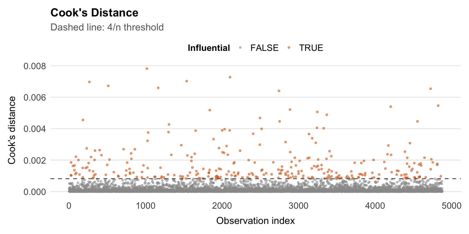
```{r}
#| label: cooks-distance
#| fig-width: 8
#| fig-height: 4
aug |>
    mutate(index = row_number(),
           influential = .cooksd > 4 / nrow(df_cc)) |>
    ggplot(aes(x = index, y = .cooksd, colour = influential)) +
    geom_point(size = 0.8, alpha = 0.5) +
    geom_hline(yintercept = 4 / nrow(df_cc), linetype = "dashed",
               colour = "grey40") +
    scale_colour_manual(values = c("FALSE" = "grey60", "TRUE" = palette_epi[["vermillion"]])) +
    labs(
        title    = "Cook's Distance",
        subtitle = "Dashed line: 4/n threshold",
        x        = "Observation index",
        y        = "Cook's distance",
        colour   = "Influential"
    ) +
    theme_epi(grid = "y") +
    theme(legend.position = "top")
```
## Variance Inflation Factors
As a final diagnostic, we check for multicollinearity using Variance
Inflation Factors (VIFs).
The VIF for predictor $j$ is:
$$VIF_j = \frac{1}{1 - R_j^2}$$
where $R_j^2$ is the $R^2$ from regressing $X_j$ on all other
predictors. It quantifies how much the variance of $\hat{\beta}_j$ is
inflated by collinearity relative to what it would be if $X_j$ were
uncorrelated with all other predictors.
- $VIF = 1$: no collinearity
- $VIF = 5$: moderate collinearity ($SE$ inflated by $\sqrt{5} \approx 2.2$)
- $VIF = 10$: high collinearity (commonly used as a threshold for concern)
```{r}
#| label: vif
car::vif(model_full)
```
::: {.callout-note title="Interpreting VIF output for categorical variables" collapse="true"}
For categorical predictors with more than two levels, `car::vif()`
returns a **Generalised VIF (GVIF)** rather than a standard VIF. The
GVIF accounts for the fact that a multi-level factor is represented by
multiple dummy variables.
To compare GVIFs across predictors with different numbers of
parameters, the adjusted value $GVIF^{1/(2 \cdot df)}$ is reported —
where $df$ is the number of degrees of freedom for that term (i.e., the
number of dummy variables). This is equivalent to the square root of
the VIF for binary predictors.
A rule of thumb: $GVIF^{1/(2 \cdot df)} > \sqrt{10} \approx 3.16$
flags a potential collinearity problem, consistent with the $VIF > 10$
threshold for continuous predictors.
:::
---
# Interpreting Coefficients
## Continuous Predictors
For a continuous predictor $X_j$, the coefficient $\hat{\beta}_j$
represents the estimated change in mean SBP for a one-unit increase in
$X_j$, with the other predictors held fixed.
For example, for age:
> "Each additional year of age is associated with a
> `r round(coef(model_full)["age"], 2)` mmHg increase in SBP, after
> adjusting for sex, race, and all social and lifestyle predictors."
That "holding all other predictors constant" language matters. These are
partial associations inside a multivariable model, not standalone or
causal effects.
## Categorical Predictors
For a categorical predictor, each coefficient is the adjusted mean
difference in SBP between that level and the reference group.
For education, with "College graduate or above" as the reference:
> "Participants with less than a 9th grade education had SBP
> `r round(coef(model_full)["educationLess than 9th grade"], 2)` mmHg
> higher than college graduates, on average, after adjusting for all
> other variables in the model."
## Log-Transformed Predictors
When a predictor is log-transformed, the raw coefficient is harder to
read directly because a one-unit increase in $\log(X)$ corresponds to
multiplying $X$ by about 2.7.
More useful interpretations:
**A doubling of $X$:**
$$\Delta Y = \hat{\beta}_j \times \log(2) \approx 0.693 \times \hat{\beta}_j$$
**A 10% increase in $X$:**
$$\Delta Y \approx \hat{\beta}_j \times \log(1.10) \approx 0.095 \times \hat{\beta}_j$$
For our physical activity variable (`log_total_met`):
> "A doubling of total physical activity (in MET-minutes per week) is
> associated with a
> `r round(coef(model_full)["log_total_met"] * log(2), 2)` mmHg change
> in SBP, after adjustment."
::: {.callout-note title="Reporting coefficients vs p-values" collapse="true"}
A common but problematic habit is to report only whether a coefficient
is "significant" (p < 0.05) rather than the estimated magnitude and
its uncertainty. Statistical significance tells you that the estimate is
unlikely to be zero by chance — it says nothing about whether the effect
is large enough to matter in practice.
**Best practice is to report:**
1. The coefficient estimate $\hat{\beta}$ (the magnitude of the effect)
2. The 95% confidence interval (the uncertainty around the estimate)
3. The p-value (the strength of evidence against the null)
For example:
| Predictor | $\hat{\beta}$ (mmHg) | 95% CI | p-value |
|---|---|---|---|
| Age (per year) | +0.40 | (0.37, 0.43) | < 0.001 |
| Non-Hispanic Black vs White | +4.93 | (3.87, 5.99) | < 0.001 |
| < 9th grade vs college grad | +5.40 | (3.21, 7.59) | < 0.001 |
This makes clear that while all three are statistically significant,
the racial disparity and education effect are of comparable magnitude,
while the age effect per year is small (though cumulative over decades
it is substantial).
Reporting only stars (***, **, *) discards the magnitude and direction
of the effect entirely — always report the number.
:::
```{r}
#| label: tbl-coefficients
tidy(model_full, conf.int = TRUE) |>
    filter(term != "(Intercept)") |>
    mutate(
        term     = str_remove(term, "^(race|education|smoking_status|food_security|sex|diabetes_flag)"),
        across(c(estimate, conf.low, conf.high), ~ round(., 2)),
        p.value  = case_when(
            p.value < 0.001 ~ "< 0.001",
            p.value < 0.01  ~ "< 0.01",
            p.value < 0.05  ~ paste0(round(p.value, 3)),
            TRUE            ~ paste0(round(p.value, 2))
        ),
        ci = paste0("(", conf.low, ", ", conf.high, ")")
    ) |>
    select(term, estimate, ci, p.value) |>
    knitr::kable(
        col.names = c("Predictor", "β (mmHg)", "95% CI", "p-value"),
        caption   = "Full model: adjusted coefficient estimates"
    )
```
---
# Limitations and Caveats
The results are useful, but they have clear limits:
**Cross-sectional design.** NHANES captures a snapshot in time. We
observe associations between SBP and social factors at one point, but
cannot infer that changes in social factors would cause changes in SBP.
Longitudinal data would be needed to make causal claims.
**Missing variables.** The most likely explanation for the model's
modest $R^2$ is unmeasured variables — particularly **antihypertensive
medication use**. Participants taking blood pressure medication will
have artificially suppressed SBP relative to their "true" underlying
level. Without controlling for this, the effects of social factors are
attenuated and their relationship to SBP is distorted.
**Complete case analysis.** Restricting to participants with non-missing
data on all variables may introduce selection bias if missingness is
related to SBP or social factors. Multiple imputation would address
this but was not used here.
**Survey design.** NHANES uses a complex stratified sampling design.
Unweighted OLS does not account for sampling weights, PSUs, or strata.
The coefficient estimates may be approximately unbiased, but standard
errors and confidence intervals may be slightly underestimated.
**Residual confounding.** Even after adjusting for 12 predictors, there
will be unmeasured variables correlated with both the social factors and
SBP. The observed associations — particularly the racial disparity —
should not be interpreted as the total causal effect.